Adaptive Single Piecewise Interpolation Reproducing Kernel Method for Solving Fractional Partial Differential Equation

DU Mingjing(杜明婧)

Institute of Computer Information Management, Inner Mongolia University of Finance and Economics, Hohhot 010070, China

Abstract: It is well-known that using the traditional reproducing kernel method (TRKM) for solving the fractional partial differential equation (FPDE) is very intractable. In this study, the adaptive single piecewise interpolation reproducing kernel method (ASPIRKM) is determined to solve the FPDE. This improved method not only improves the calculation accuracy, but also reduces the waste of time. Two numerical examples show that the ASPIRKM is a more time-saving numerical method than the TRKM.

Key words: fractional partial differential equation (FPDE); reproducing kernel method(RKM); single piecewise; numerical solution

Introduction

The focus of this study is the fractional partial differential equation (FPDE) which can be described as

(1)

whereμ(x,t),ν(x,t),ξ(x,t), andF(x,t) are known, 0<α≤1,Ω=Ωx×(0,T],Ωx=[0,1].The fractional derivative is defined in the Caputo sense shown as

(2)

There are many numerical methods for solving FPDEs. For example, Liaqatetal.[1]used the (adaptation on power series method) (AOPSM) to deal with the nonlinear PDEs. Faheemetal.[2]used a high resolution (Hermite wavelet technique) (HWT) for solving the space-time-FPDEs. Prakashetal.[3]used the (invariant subspace method) (ISM) to deal with the (m+1)-dimensional nonlinear time-FPDEs. Santraetal.[4]provided a (fresh finite difference technique) (FDT) with error estimation for solving the time-PIDE with (integro of Volterra type) (IVT). Zheng[5]used a collocation method for solving a nonlinear variable-order FDE. Wangetal.[6]used a (spectral Petrov-Galerkin method) (SPGM) to deal with the (fractional ordinary differential equation) (FODE),etc.(Reproducing kernel method) (RKM) is a new developed numerical method in recent years. Linetal.[7]gave a fresh numerical method to deal with the time-FPDEs with a space operator of general form. Postavaru and Toma[8]used a novel method for dealing with the two-dimensional FODEs by structuring a fresh set of fractional-order hybrid of block-pulse functions and Bernoulli polynomials. Yuttananetal.[9]used the (fractional-order generalized Taylor wavelets) (FOGTWs) method for dealing with the distributed-order FPDEs. Kheybari[10]used a fresh numerical method as a suitable tool which deals with the time-space FPDEs in Caputo sense by variable coefficients. Sadri and Aminikhah[11]provided a good technology for disposing the (fractional mobile-immobile advection-dispersion equations) (FMAEs). Kumar and Singh[12]used Legendre and Chebyshev wavelets to get the arithmetic solution of Black-Scholes option pricing time-FPDE. Abedinietal.[13]presented a (Petrov-Galerkin finite element method) (PGFEM) for dealing with the PDEs. Alkhalissietal.[14]used a novel (wavelet method) (WM) to solve linear or nonlinear FDEs which was presented by the generalized Gegenbauer-Humbert polynomial. Behear and Ray[15]solved the pantograph Volterra delay-integro-differential equations by a numerical (fractional integral operational matrix technology) (FIOMT) based on the Euler wavelets, and the FIOMT was presented for the pantograph Volterra delay integro-differential FDEs. Fareedetal.[16]gave a fresh high efficiency calculation method to solve FDEs with (Atangana-Baleanu operator) (ABO) technology. (Controlled Picard’s method) (CPM) is used to deal with a class of FDEs with order 0<α<1.Zhaoetal.[17]thought about a stochastic FDE and used the (Galerkin spectral method) (GSM) for solving the stochastic FPDEs. Quetal.[18]used the (neural network method) (NNM) to deal with the nonlinear spatiotemporal variable-order FPDEs. Wangetal.[19]built an effective numerical method to deal with the two-dimensional nonlinear fourth-order PDE. Dasetal.[20]dealt with the fractional Volterra integro-PDE by using Leibniz’s rule. Furthermore, the (variational iteration method) (VIM) proposed by Anjum and He[21]and the homotopy perturbation method (HPM) proposed by He[22]also could solve the FPDE.

It is reported that (traditional reproducing kernel method) (TRKM) is a new developed numerical method in recent years. Wangetal.[23-24]used the TRKM for solving the fractional problem. Duetal.[25-27]improved the TRKM by the piecewise interpolation technology. Daietal.[28]also used the (piecewise interpolation reproducing kernel method) (PIRKM) for solving the time variable fractional order advection-reaction-diffusion equations (ARDEs). The higher accuracy numerical solution by the PIRKM was obtained in Refs.[25-28]. However, the more tablets we chose, the higher absolute errors were obtained. Sometimes the absolute errors of dividing 100 and 1 000 tablets are almost the same, but the latter one requires much more work than the former one. In order to solve this complex issue, the PIRKM still need to be refined again.

This paper is constituted as follows. The reproducing kernel spaces (RKSs) and their reproducing kernels (RKs) are given in section 1. In section 2, the steps of the (adaptive single piecewise interpolation reproducing kernel method) (ASPIRKM) are presented. In section 3, the convergence analysis and its error estimate of ASPIRKM are given. In section 4, two numerical examples are presented that the ASPIRKM is a higher precision and more time-saving numerical method than the TRKM. In section 5, remarks and future directions are presented.

1 RKSs

For the sake of presentation, letΩ=[0,1]×(0,1], and the RKSs and their RKs are presented as follows.

Its inner product is

Its RK is

(3)

Its inner product is

Its RK is

(4)

Its inner product is

Its RK is

(5)

whereR(t,x) andR(x,t) are presented in Ref. [29].

its inner product is

(5) The RKS

2 ASPIRKM

The inhomogeneous conditions need to be treated as secondary conditions before solving the FPDE by the new method in the RKSs, so Eq. (1) turns to Eq. (6), andw(p,t)is the exact solution, where (p,t)∈G=[0, 1]×[0, 1], then

(6)

(7)

Using SPIRKM in Eq. (7), we set a maximum absolute error (MAE)χof [pk-1,pk]×[0,1],k=0, 1, …,n, once the absolute errors of numerical solution are bigger thanχ,[pk-1,pk]×[0,1] will go on to be single piecewise until the absolute errors of numerical solution are smaller thanχ.Then stop to be piecewise, and so on, until get the more precise results of theG.For example, in Fig. 1, we take more points in the steep interval. The two numerical examples in section 4 show that ASPIRKM has a higher precision and is a more time-saving numerical method than the old method.

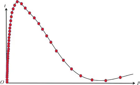
Fig. 1 Adaptive single piecewise interpolation

3 Convergence Analysis and Error Estimate

ProofFor∀(p,t)∈G，

|wn(p,t)-w(p,t)|=|〈wn(ξ,η)-w(ξ,η),K(ξ,η)(p,t)〉|≤

and theK(ξ,η)(p,t)is the RK of theH(G),∃M>0， then

ProofImplyingLw(pi,ti)=Lwn(pi,ti), we obtain

|Lw(p,t)-Lwn(p,t)|=

|Lw(p,t)-Lw(pi,ti)-(Lwn(p,t)-Lwn(pi,ti))|,

Applying the nature of RK, it has

w(p,t)=〈w(ξ,η),K(p,t)(ξ,η)〉,
Lw(p,t)=〈w(ξ,η),LK(p,t)(ξ,η)〉,

then

Lw(p,t)-Lwn(p,t)=Lw(p,t)-Lu(pi,ti)-(Lwn(p,t)-Lwn(pi,ti))=〈w(ξ,η),LK(p,t)(ξ,η)-LK(pi,ti)(ξ,η)〉-〈wn(ξ,η),LK(p,t)(ξ,η)-LK(pi,ti)(ξ,η)〉=〈w(ξ,η)-wn(ξ,η),LK(p,t)(ξ,η)-LK(pi,ti)(ξ,η)〉,

further

|w(p,t)-wn(p,t)|=|L-1(Lw(p,t)-Lwn(p,t))|≤

|〈w(ξ,η)-wn(ξ,η),L-1LK(p,t)(ξ,η)-L-1LK(pi,ti)(ξ,η)〉|≤

next

4 Numerical Examples

Example1Consider formula (1) withU(x,0)=0,U(0,t)=0 and boundary conditionU(1,t)=0, where the parameters areξ=0.1,α=0.8,μ=0.8,ν=0.01,U(x,t)=t3·sin2(πx).F(x,t) is presented byU(x,t).By numerical calculations with Mathematical 12, selectN=20.ThenU(x,t)is given in Fig. 2. Figure 3 shows the exact solutionU(x,t) (black line) and the numerical solutionsU20(x,t) (green line) with TRKM, ASPIRKM (h=0.1,χ=1), ASPIRKM (h=0.01,χ=0.1) and ASPIRKM (h=0.001,χ=0.01) att=1.

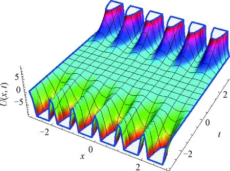
Fig. 2 U(x,t) of Example 1

Fig. 3 U20(x,t) of Example 1 by (a) TRKM; (b) ASPIRKM (h=0.1, χ=1); (c) ASPIRKM (h=0.01, χ=0.1); (d) ASPIRKM (h=0.001, χ=0.01) at t=1

Example2Consider formula (1) with theU(x,0)=sin2(2πx),U(x,t)=0 and boundary conditionU(1,t)=0 where the parameters areα=0.5,μ=0.5,ν=0.01,ξ=0.05,U(x,t)=sin2(πx)·cos2(πt).F(x,t)is presented by theU(x,t).By numerical calculations with Mathematical 12, selectN=20.TheU(x,t)is given in Fig. 4. Figure 5 gives the exact solutionU(x,t) (black line) and the numerical solutionsU20(x,t) (green line) with TRKM, ASPIRKM (h=0.01,χ=0.01), ASPIRKM (h=10-6,χ=10-5) and ASPIRKM (h=10-7,χ=10-5) att=0.8.Figure 6 shows the absolute errors |U(x,t)-U20(x,t)| by TRKM, ASPIRKM (h=0.001,χ=0.1), ASPIRKM (h=10-6,χ=10-5) and ASPIRKM (h=10-7,χ=10-6) att=0.8.

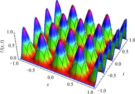
Fig. 4 U(x,t) of Example 2

Fig. 5 U20(x,t) of Example 2 by (a) TRKM; (b) ASPIRKM (h=0.01, χ=0.01); (c) ASPIRKM (h=10-6, χ=10-5); (d) ASPIRKM (h=10-7, χ=10-5) at t=0.8

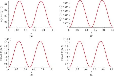
Fig.6 |U(x,t)-U20(x,t)|of Example 2 by (a) TRKM; (b) ASPIRKM (h=0.001, χ=0.1); (c) ASPIRKM (h=10-6, χ=10-5); (d) ASPIRKM (h=10-7, χ=10-6) at t=0.8

5 Conclusions

In this study, the ASPIRKM is proposed for solving the FPDEs, which combines the advantages of adaptive single algorithm and precision of the piecewise interpolation technology. By properly choosing piecewise number, we can reduce the workload and ensure the accuracy of calculation. The two numerical examples explain that the new method is a higher-precision and more time-saving numerical method compared with the TRKM. The method of this paper is also suitable for solving the nonlinear FPDEs.