Machine learning-based analyses for total ionizing dose effects in bipolar junction transistors
2022-11-21BaiChuanWangMengTongQiuWeiChenChenHuiWangChuanXiangTang
Bai-Chuan Wang· Meng-Tong Qiu · Wei Chen · Chen-Hui Wang,4 ·Chuan-Xiang Tang
Abstract Machine learning methods have proven to be powerful in various research fields. In this paper, we show that research on radiation effects could benefit from such methods and present a machine learning-based scientific discovery approach. The total ionizing dose (TID) effects usually cause gain degradation of bipolar junction transistors (BJTs), leading to functional failures of bipolar integrated circuits.Currently,many experiments of TID effects on BJTs have been conducted at different laboratories worldwide,producing a large amount of experimental data,which provides a wealth of information. However, it is difficult to utilize these data effectively. In this study, we proposed a new artificial neural network (ANN) approach to analyze the experimental data of TID effects on BJTs.An ANN model was built and trained using data collected from different experiments. The results indicate that the proposed ANN model has advantages in capturing nonlinear correlations and predicting the data. The trained ANN model suggests that the TID hardness of a BJT tends to increase with base current IB0. A possible cause for this finding was analyzed and confirmed through irradiation experiments.
Keywords Total ionizing dose effects · Bipolar junction transistor · Artificial neural network · Machine learning ·Radiation effects
1 Introduction
Bipolar junction transistors (BJTs) are widely used as analog components in electronic systems [1]. Unfortunately, BJTs exhibit total ionizing dose (TID) effects,which induce current gain degradation in radiation environments []. Such TID effects are complex and influenced by many factors. A large number of studies have been conducted on various dependences and underlying mechanics of TID effects, on bipolar devices 2–6, as well as on other types of devices [7–10]. Generally, to investigate the correlations between the TID hardness and the parameters of BJTs,a series of devices should be prepared for comparison. This method is effective in excluding the influence of other parameters, but is costly. Many laboratories worldwide have been conducting TID experiments for many years, producing a large amount of experimental data. Such data are growing rapidly and are readily available. The correlations between the TID hardness and the parameters of the BJTs may be extracted from these data.However, such highly nonlinear data cannot be accurately described using multiple linear regression. Therefore, a new generation of computational tools is needed to assist researchers in extracting valuable information from the growing volumes of data.
Machine learning methods can capture correlations in data and make predictions,thereby providing an alternative approach for scientific investigations [11]. These methods,which exhibit huge potential for generalized suitability for scientific research, have been applied to different research areas for decades [12]. Examples include genetic research[11], antibiotic discoveries [13], material design [14–16],and quantum entanglement simulations [17, 18]. Recently,machine learning methods have also been successfully applied in an increasing number of areas in nuclear physics research [19], including nuclear theories [20–22], experimental methods [23–25], accelerator science [26, 27], and nuclear data processing [28, 29]. Neural networks are powerful methods that have proven to be effective for nonlinear function fitting and accurate prediction [30, 31].
In this paper, we demonstrate that research on radiation effects could benefit from machine learning methods and present a machine learning-based scientific discovery approach for the TID effects of BJTs. Specifically, an artificial neural network (ANN) model was built and trained using the data collected from different experiments.The results indicate that the trained neural network model has significant advantages over the traditional multiple linear regression in capturing nonlinear correlations and predicting data. The trained ANN model suggests that the TID hardness of a BJT tends to increase with base current IB0. A possible mechanism for this phenomenon was analyzed and experimentally verified. Our work indicates that machine learning methods have advantages in discovering correlations and predicting experimental data. The proposed approach could be a powerful new tool to discover correlations from experimental datasets and make predictions for radiation effects.
2 Methods
2.1 Datasets
TID degradation is related to many parameters such as bias, layout, dose, dose rate, passivation layer, and hydrogen content [32–34]. A dataset containing all the related parameters is perfect for analysis. However, the collected historical experimental data do not contain all related parameters. Nevertheless, a dataset containing several parameters may still be helpful in assisting scientific discovery by providing useful information, as described herein.
The experimental dataset to be analyzed was collected from 10 articles [1, 35–43]. The Gummel-plot data of 12 bipolar devices (eight NPNs and four LPNPs) were obtained from the literature. The Gummel plot records the collector and base current values at different base-emitter voltages. Experimental data of bipolar devices irradiated by cobalt-60 gamma sources with different doses and dose rates at room temperature were collected. The Gummel plots before and after irradiation were measured. Degradations of BJTs with different types,VBE,Beta0,IB0,doses,and dose rates were extracted to create the dataset depicted in Fig. 1. The dataset contains 565 radiation response data points for two types of BJTs: NPN and LPNP. VBEis the base-emitter voltage, whereas Beta0and IB0are the corresponding common emitter current gain and base current before irradiation, respectively. The maximum dose was 1,902 krad(Si). The dose rate was in the range of 0.0015–312 rad(Si)/s.The absorbed doses and dose rates of silicon were used in this study.The degradation of a BJT is represented by the change in the base current IB/IB0,where IB0and IBare the base currents before and after irradiation,respectively. The total ionizing dose effects mainly cause an increase in the base current IBat a fixed base-emitter voltage VBE, whereas the collector current ICremains roughly constant[37,39].Therefore,IB/IB0represents gain degradation of the BJT.
In addition to the Gummel-plot data, the correlations between degradations and doses or dose rates,obtained via experimentation, have been exhibited in the literature[35, 40, 41]. These additional data were adopted as a test set to verify the generalization of the trained ANN model.None of the experimental data in the test set were used to train the ANN.
2.2 Artificial neural network model
We focused on three-layer ANNs,which have proven to be powerful in studies using relatively small datasets[44, 45]. The ANNs were implemented using a deep learning framework called Keras [46]. The inputs of the ANN are the type, |VBE|, Beta0, IB0, dose, and dose rate.The first neuron of the input layer represents the type of a BJT. Specifically, ‘0’ stands for the NPN type and ‘1’stands for the LPNP type. Each input parameter is normalized to a mean of 0 and standard deviation of 1 over the training dataset. The output of the ANN was one neuron,corresponding to the change in the base current in the logarithm log(IB/IB0).The rectified linear unit(ReLU)[47]was adopted as the activation function for the first two layers,while the linear activation function was adopted for the last layer. The dropout algorithm with the rate of 0.1 was employed for the first two layers. This algorithm is helpful in improving the generalization performance of ANNs [48]. The loss function is the mean squared error.Adam with the default learning rate of 0.001 was employed as the optimizer to update the weights during the training process [49]. The batch size was set to 32 for stable convergence during the training [50].A suitable number of neurons and training epochs may vary significantly for different problems. Fivefold crossvalidation(CV)was utilized to identify the suitable number of neurons in the two hidden layers and training epochs for fitting our dataset.In this technique,the dataset is randomly divided into five parts; five ANNs were trained and iteratively evaluated.Each ANN was trained using four parts of the dataset and validated using the remaining part.The CV technique was helpful in reducing the influence of training instability. The performance of the ANNs was evaluated using the mean absolute error (MAE), computed as:

Fig.1 Overview of the dataset:degradation log(IB/IB0)versus(a)type,(b)bias condition VBE,(c)common emitter current gain Beta0,(d)base current IB0, (e) dose, and (f) dose rate

where y and ^y represent the experimental and predicted values for log(IB/IB0), respectively, and N represents the number of data points.
The performance of the ANNs with different training epochs and neuron numbers is shown in Fig. 2. The training and validation MAEs are the average values of all five-fold ANNs. The maximum number of neurons to be investigated was limited to 20 × 20 considering the small size of the dataset to be fitted.As can be seen in Fig. 2a,the MAE on the validation set converged after 1,000 epochs of training for the different sizes of ANNs evaluated in our study.Therefore,the number of epochs for training was set to 1,000.Figure 2b presents the influence of the number of neurons in the two hidden layers on the valid MAE. The MAE on the validation set decreased with an increase in neurons.The distribution of the MAE is symmetrical about the diagonal. Therefore, it is a good choice to set the number of neurons in the two layers equal when the total number of neurons is fixed. Figure 2c shows the MAEs of the training and validation sets for ANNs with the same number of neurons in the two layers. As the number of neurons increased,the MAEs of the training and validation sets decreased. However, the MAE of the validation set decreased more slowly than that of the training set. As shown in Fig. 2d,the difference between the two increased.A large difference indicates that the model can fit the training set accurately, but cannot accurately predict the validation set. This indicates poor generalization performance owing to overfitting [51]. To accurately capture the correlations between data, a good model should have a small MAE and a good generalization performance.In our study, we set the number of neurons in each layer to 7.Figure 3 displays a schematic of the proposed ANN model.Applying more neurons could reduce the MAE slightly,but simultaneously reduces the generalization performance.We preferred fewer neurons to avoid capturing fake correlations caused by overfitting.
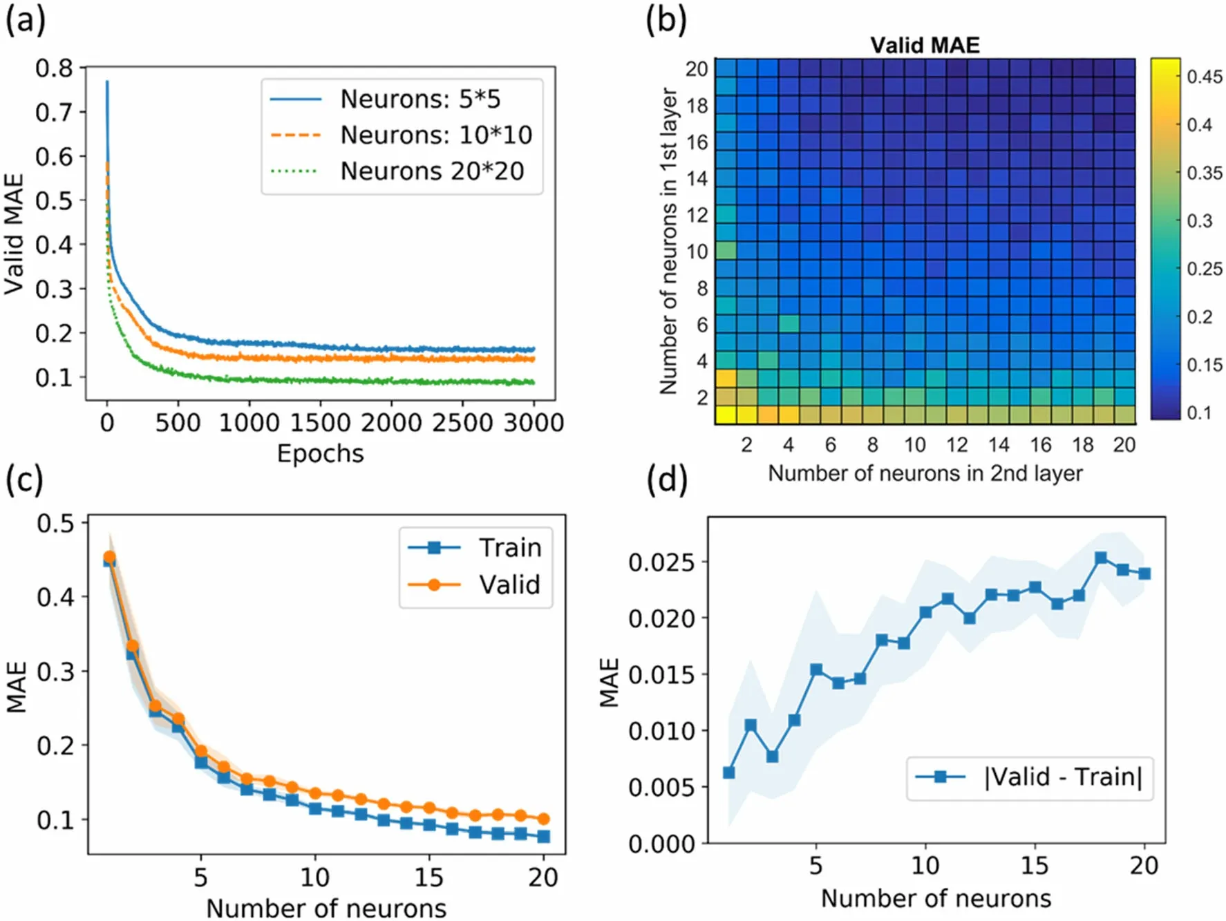
Fig. 2 Performance of ANNs with different training epochs and numbers of neurons.(a)Valid MAE for different training epochs.The valid MAE converges after 1,000 epochs for ANNs with different numbers of neurons.(b)Valid MAE for ANNs with different numbers of neurons in two hidden layers.(c)Training MAE and valid MAE for ANNs with the same number of neurons in the two layers.(d) Differences between training MAE and valid MAE. For (c) and(d),the data points in the figures are the average values of 10 random runs, while their standard deviations are marked with shaded areas.(Colour figure online)

Fig. 3 Schematic of the proposed ANN model for our dataset.(Colour figure online)
3 Results
3.1 Predictions
With the help of CV technology, five ANNs were trained using different parts of the dataset.The predictions made by these ANNs were slightly different. We used the average value as the prediction result. The performance of the trained ANNs regarding the test set is expressed in Fig. 4.Figure 4a–g shows that the degradations at different doses and dose rates predicted by the trained ANN model agree with the experimental results for the test set. Figure 4h presents a summary of the predictions for the test set. The MAE between the predictions and experimental data was 0.101.
Figure 5 presents a comparison of the learning curves for the three different models. The performance of our proposed ANN model was compared with those of the average and multiple linear regression models.The average model considers the average value of the training set samples as the prediction results.As the number of training samples increased, the MAE on the test set decreased significantly for the ANN and multiple linear regression models.When trained with 550 samples,the average MAE for 10 random runs of the ANN model was the smallest,which was nearly half of that of the multiple linear regression model.The results show that the proposed ANN model performs better than the traditional multiple linear regression model in predicting the experimental results.

Fig. 4 Performance of the trained ANN model on the test set: (a)–(g) Experimental results and predictions of degradations at different doses and dose rates. (h) Summary of the predictions for the test set.Error bars represent the standard deviations of different CV parts.(Colour figure online)

Fig. 5 Comparison of learning curves for average model, multiple linear regression, and ANN. The data points in the figures are the average values of 10 random runs,while their standard deviations are marked with shaded areas. (Colour figure online)
3.2 Correlations
The trained ANN model fits the experimental data well,indicating that the trained ANN model successfully learned the correlations between the degradation and input parameters in the dataset. These correlations were investigated by feeding the trained ANN model with specific inputs. Figure 6 displays the correlations between the degradation and each parameter generated by the trained ANN model. Specifically, dose = 100 krad(Si), dose rate = 100 rad(Si)/s, |VBE| = 0.6 V, Beta0= 100, and IB0-= 1 × 10⁻⁸A were selected as the reference parameter values.The data points in the figures are the average values of the different CV parts, and the shaded areas represent their standard deviations. The correlations captured via multiple linear regression are shown in Fig. 7 for comparison.
Most correlations captured by the trained ANN model were consistent with classical theories, whereas a novel correlation was found.These correlations are nonlinear and cannot be accurately described using multiple linear regression model. In Fig. 6a, the degradation trend with dose is shown. It is apparent that the degradation of the BJT increases with increasing dose before saturation. In particular, degradation of the LPNP-type BJT was more severe and saturated earlier. These phenomena are consistent with those reported in previous studies [35]. As depicted in Fig. 6b, the degradation at a low dose rate is more severe, implying that enhanced low dose rate sensitivity (ELDRS) effects are captured in the ANN model.Figure 6c indicates the consistency with previous research results that degradation is more severe at lower bias voltages [1]. In Fig. 6d, the captured correlation between degradation and Beta0is unclear. It seems that for the NPN-type device, the degradation increased with Beta0.However,the degradation changed little with Beta0for the LPNP-type. In Fig. 6e, it is noteworthy that the trained ANN model captured the correlation that degradation of a BJT will lessen as the pristine base current IB0increases,that is, the TID hardness of a BJT tends to increase with base current IB0. To the best of our knowledge, this hypothesis has rarely been reported in the literature.
The proposed hypothesis shown in Fig. 6e agrees with the statistical analyses. The pristine base current IB0and VBEare related. To exclude the influence of VBE, the experimental data of the same bias (VBE= 0.6 V) were selected to analyze the correlation between IB0and the
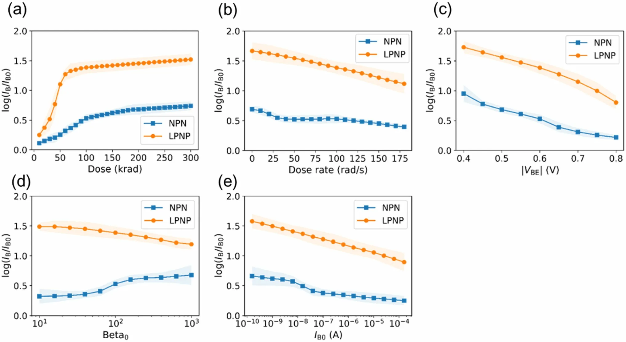
Fig. 6 Correlations captured by the trained ANN model between the degradation and each parameter.(a)–(e)results from the trained ANN model with the reference parameters: dose = 100 krad(Si), dose rate = 100 rad(Si)/s, |VBE| = 0.6 V, Beta0 = 100, and IB0 = 1 × 10⁻⁸ A. Shaded areas represent the standard deviations of different CV parts. (Colour figure online)
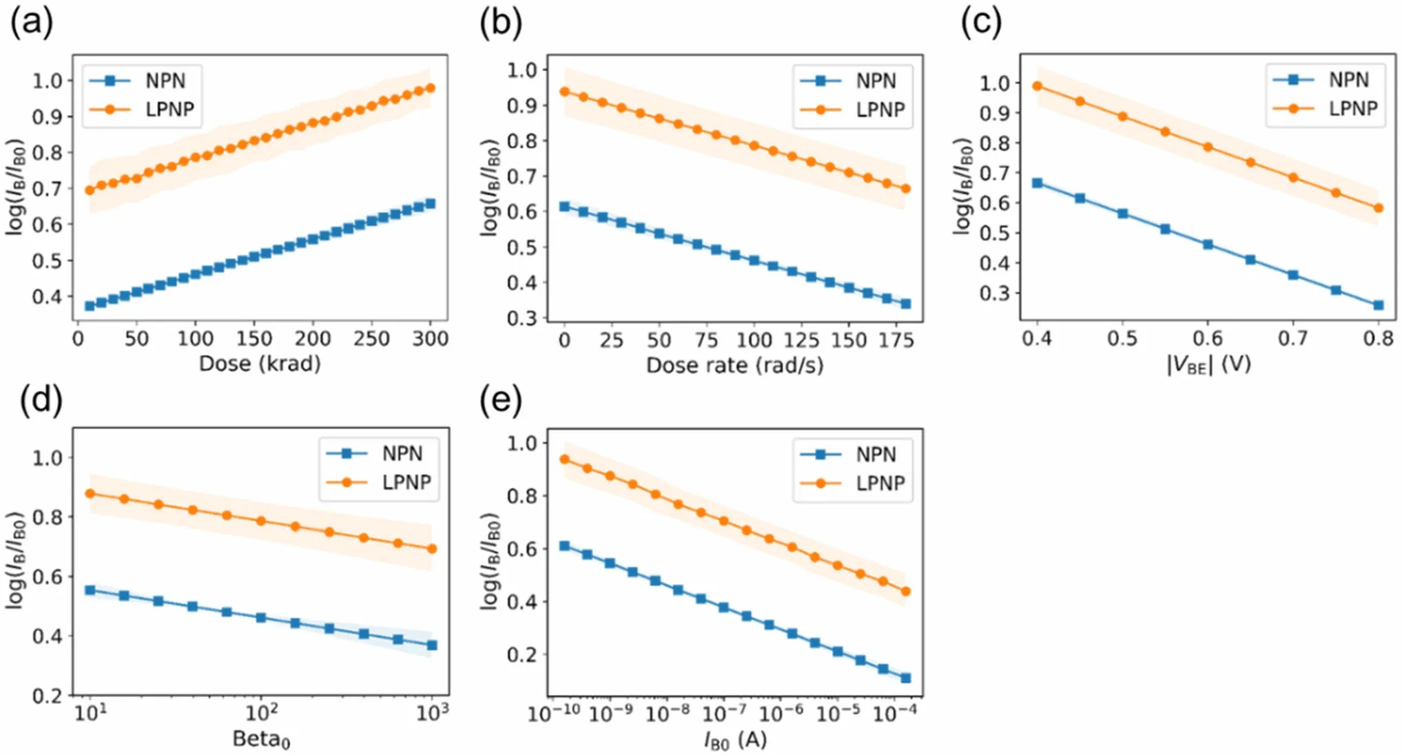
Fig. 7 Correlations captured by the multiple linear regression model between the degradation and each parameter. Shaded areas represent the standard deviations of different CV parts. (Colour figure online)

3.3 Mechanism analyses
The possible causes of the proposed hypothesis could be analyzed using classical TID mechanism theories. For an ideal NPN BJT, the pristine base current can typically be approximated as:

where PEis the emitter perimeter, Δs is the surface recombination velocity, niis the intrinsic carrier concentration of silicon, and Emis the maximum electric field in the SCR [53]. The excess base current in the NBS is expressed as:
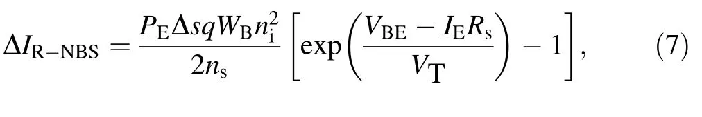
where nsis the majority carrier concentration at the surface and WBis the width from the emitter to collector [53, 55].The degradation can be written as:

Notably, the total excess base current ΔIR, which is the sum of ΔIR-SCRand ΔIR-NBS, is proportional to the perimeter of the emitter PE.The pristine base current IB0is proportional to the area of the emitter A. When other parameters of the BJTs are approximately the same, the degradation should be proportional to the perimeter-to-area ratio, that is:

The perimeter increased as the area of emitter A increased, but the perimeter-to-area ratio (PE/A) tended to decrease. Consequently, IB/IB0decreased. Therefore, the difference in the perimeter-to-area ratio PE/A may be one of the possible mechanisms leading to the phenomenon that a BJT with a larger base current IB0tends to have a smaller degradation IB/IB0.
3.4 Irradiation experiments
Irradiation experiments were conducted to verify the influence of the perimeter-to-area ratio on degradation.The irradiation experiments were performed using a cobalt-60 gamma source at room temperature. Five kinds of NPN BJTs with different emitter sizes were irradiated,as shown in Fig. 8a. The other parameters of the BJTs are approximately the same. The devices were manufactured by Analog Foundries, based on a 6-inch bipolar process platform. Accounting for the uncertainties caused by manufacturing process fluctuations, three devices of each kind were used for irradiation.The total doses were 40,80,120,and 160 krad(Si), and the dose rate was 0.685 rad(Si)/s in the experiments. All BJTs were grounded during irradiation. The Gummel-plot data were measured using a semiconductor analyzer at room temperature before and after irradiation. VEwas swept from - 0.4 to - 1.2 V, maintaining VB= VC= 0 V. The delay between irradiation and every measurement was within 2 h. Typical Gummel-plot data at different doses are presented in Fig. 8b.
As shown in Fig. 8c, the degradation IB/IB0increases linearly with the perimeter-to-area ratio PE/A,which agrees with Eqs. (8) and (9). The measured correlations between the degradation and pristine base current at different doses,shown in Fig. 8d, indicate that a BJT with a larger base current IB0tends to have a smaller degradation IB/IB0,which is consistent with the ANN result. Experiments confirmed that the perimeter-to-area ratio could be one of the causes of this phenomenon.

Fig. 8 Results of the irradiation experiments. (a) Emitter sizes of BJTs used in experiments. (b) Gummel plots for one of the 18 × 18 μm2 emitter BJTs at different doses. (c) Degradation versus perimeter-to-area ratio at different doses (VBE = 0.6 V). Error bars are the standard deviations of the measurement results. Dashed lines are the linear fitting results of the mean values.(d)Degradation versus pristine base current at different doses (VBE = 0.6 V). (Colour figure online)
4 Discussions
4.1 Predictive ability
It should be noted that the trained ANN cannot guarantee the degradation prediction for a device that does not have any data in the training set. This is because of the systematic deviations between different devices and experiments. An ANN may overestimate or underestimate a device that has never been observed.The trained ANN is more suitable for predicting missing values, such as predicting degradations at other doses or dose rates in Sect. 3.More specifically, the ANN was trained to predict missing values in the training process. The dataset included experimental data from different devices. During training,the dataset was shuffled and divided into training and validation sets. The validation set can be considered the missing value of the training set. The ANN model was trained using the training set and verified by predicting the validation set.Therefore,the performance of the validation set correlates with ANN’s ability to predict missing values.
As shown in Fig. 9a,the ANN failed to predict the data from the irradiation experiments in Fig. 8.The degradation was overestimated and the MAE was as large as 0.45.However, after the 130 krad Gummel-plot data of the 18× 18 μm2NPN were included in the dataset, the predictions of the newly trained ANN model on irradiation experiments could be significantly improved. As shown in Fig. 9b, the MAE decreased to 0.14. It is noteworthy that only the degradations at 130 krad of one device were included in the dataset, but the predictions of 9 × 9,9 × 18,18 × 18,18 × 36,and 18 × 72 μm2NPNs at 40,80,120,and 160 krad were improved.This implies that the ANN model learned the correlations from the other devices in the dataset. When more data are included, predictions can be further improved. Figure 9c shows the predictions after 50 krad Gummel-plot data of the 18 × 72 μm2NPN were added to the dataset.MAE reduced to 0.09.Note that all of the experimental data to be predicted in Fig. 9 have never been used for training.
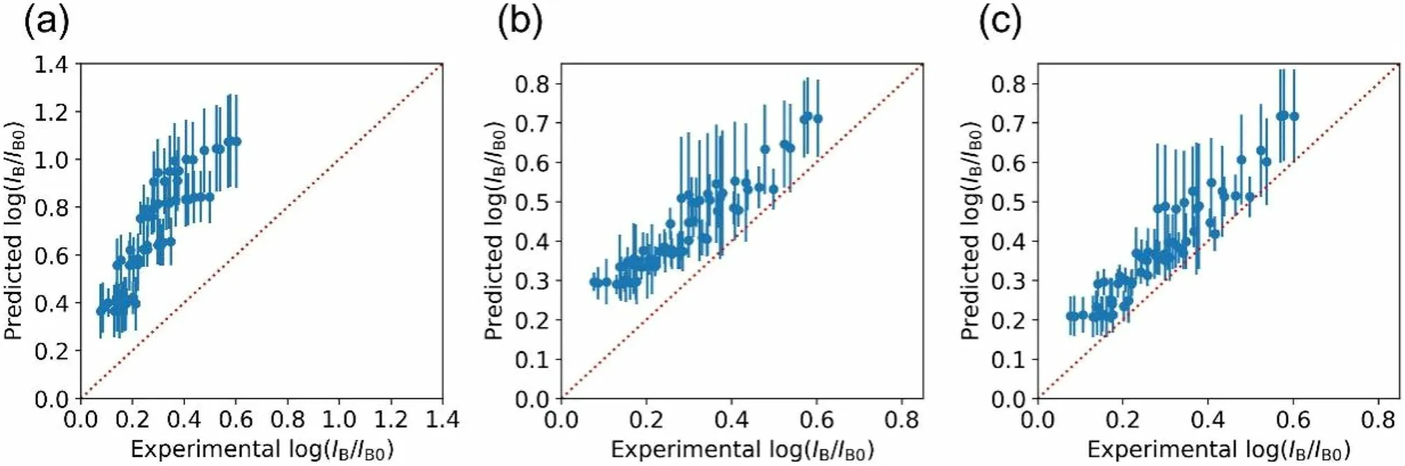
Fig. 9 Performance of predictions on experimental data of Fig. 8.(a) ANN trained with original dataset. (b) ANN trained with dataset adding 130 krad Gummel-plot data (18 × 18 μm2 NPN). (c) ANN trained with dataset adding 130 krad Gummel-plot data(18 × 18 μm2 NPN) and 50 krad Gummel-plot data (18 × 72 μm2 NPN)

Fig.10 Predictions on irradiation experiments of ANN trained with a new feature factor F. (a) Predictions versus experimental results in Fig. 8.(b)Degradations versus pristine base current at different doses(VBE = 0.6 V). Shaded areas represent the standard deviations of different CV parts. (Colour figure online)
4.2 Systematic deviations between different devices
There may be systematic deviations between different experiments, such as differences between the radiation sources and measurement instruments. Moreover, devices from different manufacturers may also exhibit systematic deviations.Systematic deviations limit the ability to predict new devices.If we could account for systematic deviations,the predictions of the new devices could be improved.
We propose a simple method for approximately characterizing the system deviations between devices. We introduced a factor F to represent the deviation of one device from the average value of the other devices. To evaluate the factor F, a multiple linear regression model was trained using the dataset, excluding the device to be evaluated. The trained model represents the average of the other devices.The predictions of the device to be evaluated are denoted by ^y, and the actual degradations are denoted by y. Factor F was calculated by linear fitting as follows:
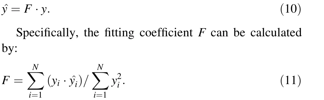
If the factor F of a device is larger than 1, the device is likely to have less degradation than the other devices in the dataset. The calculated F for the 12 devices in the dataset ranged from 0.36 to 1.48.The calculated F value was set as a new feature of the dataset to account for systematic deviations. A new ANN model with the same structure as the previous model was trained, and the predictions of our irradiation experiments are shown in Fig. 10.It is clear that this model can accurately predict the experimental results.However, the factor F of the device is required when predicting. This implies that one should have some device data to compute factor F in advance.In our case,the factor F was calculated with degradations at 130 krad.
5 Conclusion
We presented a machine learning-based scientific discovery approach for radiation effect research. It is shown that the machine learning method could be a powerful new tool to discover correlations from experimental datasets and make predictions. An ANN model was built and trained using the dataset collected from different experiments. The results indicate that the proposed ANN model has advantages over multiple linear regression in capturing most nonlinear correlations and predicting data. Most correlations captured by the trained ANN model were consistent with classical theories, whereas a new correlation was found. The trained ANN model suggests that the TID hardness of a BJT tends to increase with base current IB0. Further mechanistic analyses and experiments confirmed that the differences in the emitter perimeter-to-area ratio of the BJTs could be one of the causes of this phenomenon. The ANN model presented in this study was trained using a relatively small and simple dataset. It is expected to be more powerful if a larger and more detailed dataset is provided. We plan to conduct ANN analyses on the historical data from several laboratories and build models for other kinds of devices.
Author contributionsAll authors contributed to the study conception and design. Material preparation, data collection, and analysis were performed by Bai-Chuan Wang, Meng-Tong Qiu, and Chuan-Xiang Tang. The first draft of the manuscript was written by Bai-Chuan Wang and all authors commented on previous versions of the manuscript. All authors read and approved the final manuscript.
杂志排行

Nuclear Science and Techniques的其它文章
- Thermal hydraulic characteristics of helical coil once-through steam generator under ocean conditions
- Lifetime estimation of IGBT module using square-wave loss discretization and power cycling test
- Optimization of the cavity beam-position monitor system for the Shanghai soft X-ray free-electron laser user facility
- A beam range monitor based on scintillator and multi-pixel photon counter arrays for heavy ions therapy
- Research on manufacture technology of spherical fuel elements by dry-bag isostatic pressing
- Beam–beam effects and mitigation in a future proton–proton collider