Lifetime estimation of IGBT module using square-wave loss discretization and power cycling test
2022-11-21JieWangDaQingGaoWanZengShenHongBinYan
Jie Wang· Da-Qing Gao · Wan-Zeng Shen· Hong-Bin Yan
Abstract The insulated gate bipolar transistor (IGBT)module is one of the most age-affected components in the switch power supply, and its reliability prediction is conducive to timely troubleshooting and reduction in safety risks and unnecessary costs. The pulsed current pattern of the accelerator power supply is different from other converter applications;therefore,this study proposed a lifetime estimation method for IGBT modules in pulsed power supplies for accelerator magnets. The proposed methodology was based on junction temperature calculations using square-wave loss discretization and thermal modeling.Comparison results showed that the junction temperature error between the simulation and IR measurements was less than 3%. An AC power cycling test under real pulsed power supply applications was performed via offline wearout monitoring of the tested power IGBT module. After combining the IGBT4 PC curve and fitting the test results,a simple corrected lifetime model was developed to quantitatively evaluate the lifetime of the IGBT module,which can be employed for the accelerator pulsed power supply in engineering.This method can be applied to other IGBT modules and pulsed power supplies.
Keywords IGBT module · Junction temperature · Power cycling test·Lifetime prediction·Power loss discretization
1 Introduction
The Heavy Ion Research Facility in Lanzhou(HIRFL)is a multifunctional cooling storage ring (CSR) system [1].The HIRFL requires a stable,high-current,and high-energy beam for the CSR main ring (MR)to perform high-quality physical experiments[2].Such a large synchrotron requires a significant number of power supplies to provide a highprecision and low-ripple current for magnets. The power supplies include switching DC and pulsed power supplies[3], and numerous insulated gate bipolar transistor (IGBT)modules are employed as switching devices.The statistical data of the power supply system of the HIRFL over the last five years were studied;with the long-term operation of the equipment, faults caused by component quality and aging accounted for 33.92% and the IGBT fault time accounted for 63.22% of the total fault time. Therefore, it is imperative to investigate the reliability of IGBT modules operating under pulsed current conditions.
For the switching DC power supply,the power loss and junction temperature remained steady; hence, the IGBT module was reliable.However,the switching pulsed power supply exhibited considerable power swings and junction temperature variation, which contribute to the reduction in the IGBT module reliability. The reference pulsed current pattern of the accelerator power supply has a particular effect on the IGBT module lifetime. Few studies have evaluated IGBT module reliability for an accelerator pulsed power supply. Hence, this study aimed to present a complete solution for the lifetime estimation of an IGBT module in an accelerator pulsed power supply.
Hillman et al. [4] presented important power supply operational statistics and described an approach for meeting reliability goals.Bellomo et al. [5] performed a failure mode and effect analysis on a standard SLAC quadrupole magnet system and assisted in distinguishing the less reliable components. Siemaszko et al. [6] studied several reliability models applied to a power system, enabling estimation of reliability and availability. Reliability improvements owing to oversizing and redundancy have been identified [7]. Further, a calculation method for the junction temperature of an IGBT module for the DC model has been presented [8]. In the fields of wind power converters [9], modular multilevel converters [10], and highvoltage direct current transmission [11], the reliability of high-power IGBT devices has been widely studied,including lifetime prediction, condition monitoring, fault diagnosis, and junction temperature management.
From statistics, high temperature was found to be the predominant cause of power electronic device failure [12].The junction temperature of a device is usually limited to a safe range during operation; however, overload, high switching frequency, insufficient heat dissipation, and excessive gate resistance may lead to a high junction temperature and the failure of power semiconductor devices. The temperature profiles of power semiconductor devices constitute both nonperiodic and periodic profiles.The periodic temperature fluctuations of a power device include low-frequency, fundamental frequency, and highfrequency temperature fluctuations [9]. The low-frequency junction temperature fluctuation (typically a few seconds)caused by the periodic pulsed current is the most important factor in the aging failure of an IGBT module.
The main methods currently used to estimate the junction temperature include simulation methods,i.e.,the finite element(FE)method[13]and electrothermal coupling simulation [14], and measurement methods, i.e., fiber optic and infrared cameras.In addition,temperature-sensitive electricalparametersreflectjunctiontemperatureinformation,such as the collector–emitter voltage and threshold voltage[15].Square-wave pulse loss transforms the loss profiles into thermal profiles[16];this is a primordial method for calculating the convolution of transient power losses and thermal impedance,and the accuracy and computation quantity need to be considered.In this study,the trapezoidal power loss was dividedintonumeroussquarepowerpulses,andtheminimum amount of calculation and maximum error were determined.
The design of the power device lifetime is crucial in practical applications. An empirical lifetime model was established through numerous accelerated power cycling tests,divided into AC and DC power cycling tests.The AC power cycling test is closer to the normal operating situation;however, direct extraction of the aging characteristic parameters is difficult [17]. In this study, an AC power cycling test under real pulsed power supply applications was performed via offline wear-out monitoring of a tested power IGBT module. A simple corrected lifetime model was developed to quantitatively evaluate the lifetime of the IGBT module, which can be employed as an accelerator pulsed power supply inengineering.Thiscan assist inthe designand maintenance of a pulsed power supply.
The remainder ofthis paper isorganizedas follows.Power loss discretization and thermal modeling are detailed in the next section.As described in Sect. 3,we performed an AC power cycling test under real pulsed power supply applications,and the results were fitted to obtain a simple corrected lifetime model. Section 4 presents the experimental verification of the junction temperature,and the IR measurement results demonstrated the effectiveness of thermal modeling.Section 5 outlines the prediction of the lifetime of an IGBT module under two typical current waveforms, as well as analyses of the influence of the electrical parameters and heatsink on the IGBT module reliability.
2 Thermal modeling
2.1 Discretization of trapezoidal power loss
The working mode of an accelerator power supply is unique; it works in the frequency-doubling chopper mode and outputs a DC or pulsed current. Figure 1 shows a typical current waveform of a quadrupole magnet pulsed power supply.The pulsed current waveform(black)can be approximated as a trapezoidal waveform (orange). The device power loss is a trapezoidal wave, which is divided into four stages:rising,flat top,falling,and flat bottom.t1,t2, t1, and t3are the times for each stage. The rates of increase and decrease are equivalent.
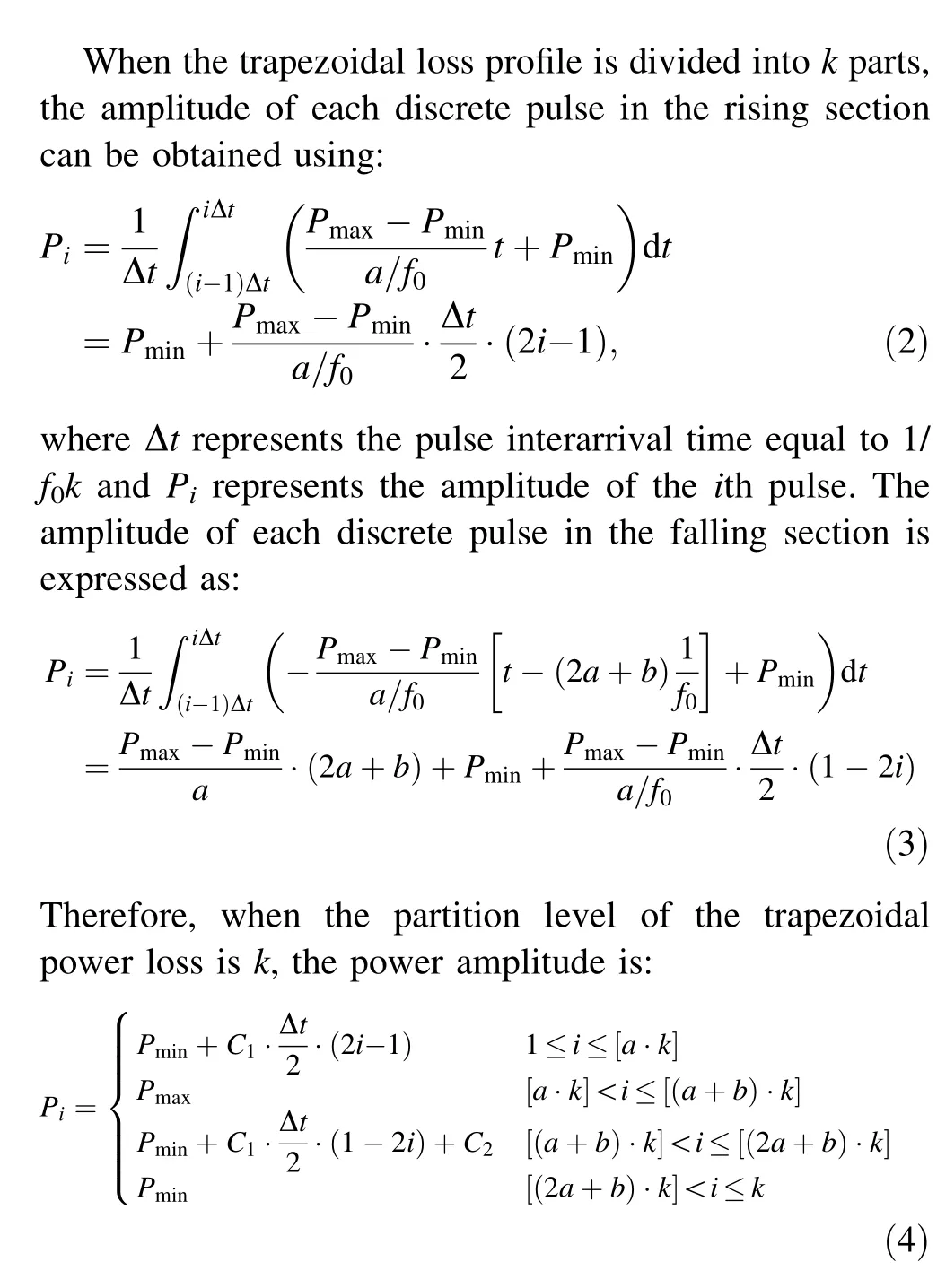
As observed in Fig. 1, the trapezoidal power loss is divided into multiple square-wave pulses,where Plossis the power loss of the IGBT module including conduction loss and switching loss; P1, P2, …, Pkare the discrete squarewave power pulses; and k is the classification level. When the divided pulse is narrower, the energy of the divided pulse is closer to the energy of the trapezoidal power loss.A one-level discrete pulse with k = 1 is expressed as:

where Pmaxand Pmindenote the flat-top and flat-bottom values of the power loss, respectively, P1denotes the amplitude of the square-wave loss, Pavedenotes the average power loss, f0denotes the frequency of the periodic current and the power loss, and a and b are the ratios of t1and t2to 1/f0, respectively.

Fig. 1 Power loss profile and discretization results: a output current; b power loss; c one-level square-wave loss; and d k-level square-wave losses
where C1and C2are constants for simplicity of expression,written as: C1= (Pmax-Pmin)f0/a, C2= C1(2a + b)/f0.
2.2 Junction temperature calculation
The IGBT module has a sandwich structure,including a chip layer, solder layer, copper layer, and ceramic layer,among others.The power loss is transferred to the heatsink through various layers of materials and is brought out through the cooling water. Thermal resistance and heat capacity are used to describe heat conduction according to the similarity between thermal and electrical engineering.The thermal impedance network of the IGBT module generally comprises multiple independent resistor–capacitor(RC)units and converts the power loss to a temperature difference. Specifically, the thermal impedance network constitutes the thermal impedance from junction to case Zthjc, the thermal impedance from case to heatsink Zthch,and the thermal impedance from heatsink to ambient Zthha.
The conversion from the power loss to the thermal profile is depicted in Fig. 2. For two power dissipation pulses,P1and P2,the junction temperature fluctuation was calculated using [18]:

Fig. 2 Junction temperature curves obtained for a two power pulses and b multiple power pulses

where P1and ΔT1are the power loss and temperature at Δt,respectively; thermal resistance Rthand time constant τthconstitute an RC combination of the heat transfer; P2and ΔT2are the power loss and temperature at 2Δt, respectively. The junction temperature change at moment iΔt is calculated in the same way as for the two power pulses.Thus, for i power pulses, the junction temperature fluctuation is calculated using:

The temperature reaches a maximum at a pulse time of[(a + b)k] + 1.

where T0denotes the ambient temperature; ΔTthjc, ΔTthch,and ΔTthhaare the temperature differences from junction to case, case to heatsink, and heatsink to ambient, respectively. Accordingly, the maximum and minimum junction temperatures were obtained.
The calculation error of the junction temperature decreases with an increase in the divided level k, but a sufficiently accurate division will lead to computational complexity. The timescale of the thermal impedance is above 1 ms[16];therefore,the pulsed interval Δt = 1 ms is considered as the appropriate value in this study. In addition, k*= 1000/f0.
The relative error of estimated temperature is given by:

3 Power cycling test methodology and results
3.1 Accelerated power cycling test setup
The lifetime model of the IGBT module can be divided into physical and empirical models.The aging process of a device is regarded as a physical or chemical process in the physical lifetime model.The damage model obtained using the plastic and creep strains of materials must be combined with FE analysis. The empirical lifetime model adopts a statistical principle to establish a model between the number of cycles to failure and external conditions.Accelerated power cycling is an important test for establishing a lifetime model. Most reliability evaluations have been performed with theoretical estimations and are separate from power cycling tests. As described herein, an AC power cycling test under realistic electrical conditions was performed, and the test results with 600-A 1200-V IGBT modules were used to develop simple corrected lifetime model parameters.

Fig. 3 (Color online) Configuration of the power cycling test setup
Figure 3 presents the configuration of the accelerated power cycling test setup based on a quadrupole magnet pulsed power supply.Accordingly,six constituent parts can be seen:voltage source,DC-link capacitor,IGBT modules,filter inductor,filter capacitor,and quadrupole magnet.The quadrupole magnet power supply operates in double frequency chopper mode, adopts a full bridge topology, and comprises two half-bridge modules (Infineon FF600R12ME4). When the power supply outputs a pulsed current, V1 and V4 switch on and off, and VD2 and VD3 are used for freewheeling.
The parameters of the AC power cycling test are listed in Table 1. Module-1 and module-2 in the pulsed power supply produce the same power loss and junction temperature fluctuation and endure the same electrical–thermal stress. The maximum estimated junction temperature Tjmax_estbefore the compensation was approximately 101 °C, and the minimum estimated junction temperature Tjmin_estwas approximately 57 °C.Tjmax_IRmeasured using an IR camera was approximately 100.29 °C,while Tjmin_IRwas approximately 57.54 °C.
According to existing research [17], the on-state saturation voltage VCEbetween the collector and emitter of the IGBT module is selected as a characteristic parameter reflecting the aging state, and an increase in VCEof 5% is considered as the judgment criterion of failure. VCEof the IGBT is measured offline by the circuit shown in Fig. 3.The driving signals of V1 and V4 were connected with a constant 15 V and the tubes were conductive;therefore,the circuit became a current path.
The experiment was accomplished as follows:the initial on-state saturation voltage change rate ΔVCEwas set to 0,the initial on-state saturation voltage VCE1was measured,and then ΔVCEwas determined as greater or less than 5%.If ΔVCEwas greater than 5%, the power cycling test wasterminated. Otherwise, 25,000 cycles of the power cycling test were performed,the present on-state saturation voltage VCE2was measured,and the new voltage change rate ΔVCEwas calculated. This process was repeated until the failure criterion was reached, which was increased by 5%. The voltage measurement points were led out through the wires.

Table 1 Power cycling test conditions
3.2 Test results
Figure 4a depicts the relative variation in VCEfor the two IGBT modules during the power cycling test, where the red arrows indicate the failure points. In this test,there was a slight increase in VCEbefore 7 × 10⁵cycles. From 9 × 10⁵to 2.5 × 10⁶cycles, the value of VCEwas stable.Subsequently, it suddenly increased. After approximately 2.55 × 10⁶cycles, the saturation voltage of module-1 increased by more than 5% from the initial value. After approximately 2.68 × 10⁶cycles,the saturation voltage of module-2 increased by 5%. Degradation of the IGBT modules was realized, and the power cycling test was completed. Therefore, the number of cycles until failure was N1= 2.5 × 10⁶and N2= 2 × 10⁶.
The power cycling capability of power semiconductor modules is mostly modeled by the Coffin–Manson law, in which the number of cycles to failure(Nf)is assumed to be proportional to ΔTjn[19] (ΔTjrepresents the junction temperature fluctuation per power cycle), expressed as:

This appears as a straight line when plotting log(Nf) over log(ΔTj). As shown in Fig. 4b, the blue curve represents the IGBT4 1200 V industrial model PC curve at Tvjmax-= 125 °C. log(Nf) and log(ΔTj) can be approximated by a linear function with the slope of - 6.9062.Combined with the slope, the test results were fitted to obtain a simple corrected lifetime model for quantitatively evaluating the lifetime of an IGBT module. The values of α and n are α = e40.886= 5.7091 × 10¹⁷and n = - 6.9062, respectively. The corrected Coffin–Manson model is written as:
Small bubbles were observed inside the failed modules after the experiments. The appearance of bubbles impacts IGBT modules and can cause unstable performance. If the module continues to operate, more serious failures will occur, including bond wire deformation, solder layer delamination, and core melting. Owing to the different thermal expansion coefficients of the materials in each layer inside the IGBT module, the materials in each layer were aged under the impact of accumulated thermal stress.
4 Verification of junction temperature
Several methods are used for measuring junction temperature. A negative temperature coefficient resistor is usually packaged inside an IGBT module; however, it cannot accurately measure the junction temperature because of its distance from the IGBT chip. Thus, a thermocouple is used with a response speed of seconds and a long response time, which is suitable for monitoring the substrate temperature of a module. A test bench for the IGBT junction temperature for an infrared camera was established on a quadrupole magnet power supply. The IR camera (FLIR E60) had the accuracy of ± 2 °C or ± 2%and produced sensitive images. The frame frequency of temperature sampling was set to 30 Hz. This noncontact temperature measurement from an IR camera exhibits a high spatial resolution.

Fig.4 Power cycling test results and Nf–ΔTj curve.a Results of accelerated power cycling tests and b fitting curves obtained from power cycling tests
Two half-bridge IGBT modules were employed. The module for observing Tjhad an open packaged structure without silicon gels and was sprayed with black paint to achieve consistent emissivity of the tested area. The detachment of silica gel affected the power insulation performance of the IGBT module. In the experiment, the rated voltage of the module was 1200 V while the actual front voltage was 50 V. The operation is considered safe.The IGBT module comprised six IGBT chips and six antiparallel diode chips. Three IGBT chips and three diode chips comprised an IGBT tube. A program was developed to determine the junction temperature.As shown in Fig. 5a,the three yellow rectangles were analyzed as the active part of the measured IGBT chip under testing. The average temperature of the three measured areas was considered to be the junction temperature. Figure 5b shows the temperature distribution in a frame.
The junction temperature results under different switching frequencies are provided in Fig. 5c,d,where the estimated temperatures for k = 5,10,and k*are illustrated.The junction temperature, Tj, oscillates at a low frequency with a constant amplitude. The estimated temperatures agreed well with the measured values. As the number of divisions increased, the error decreased, and the estimated junction temperature became closer to the experimental temperature. When T0= 3.25 s and k*= 3250, the power loss had an optimal division.The estimated thermal profile was similar to the experimental profile. The estimation errors of the thermal modeling method are listed in Table 2.When the switching frequency was 12 kHz, the estimated temperature error at k = 10 was less than 5%,whereas that at k = 5 was more than 10%. When k*was considered,the error compared with the experimental result was within 3%,proving that the proposed thermal modeling method is effective with good computational accuracy.
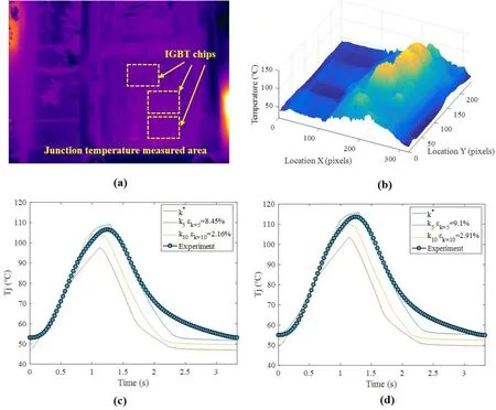
Fig.5 Infrared image and periodic junction temperature profiles with two different switching frequencies.a Image of IGBT module under test;b temperature distribution at a frame; c fs = 12 kHz; and d fs = 16 kHz

Table 2 Estimation errors of the thermal modeling method
5 Lifetime prediction
5.1 Lifetime analysis under two operating conditions
Figure 6 displays a flowchart of the lifetime estimation,including the aforementioned details.It is divided into two stages: one comprises power loss discretization and junction temperature computation of a square-wave pulse,while the other involves an accelerated power cycling test and result processing. The junction temperature is the core factor in the proposed lifetime prediction scheme, as verified in the previous section. For applications involving a trapezoidal pulsed current, a more practical set of parameters was selected to estimate the lifetime.
In practice, an accelerator pulsed power supply outputs various pulsed currents with different parameters. Two typical working conditions were selected from multiple operating pulse conditions: small and large pulsed period and current amplitude. The parameters of the two current waveforms are detailed in Table 3, including the rising time, falling time, flat-top time, flat-bottom time, turning time, flat-bottom current, and flat-top current. The pulsed periods were 7 and 17 s, and the corresponding values of the flat-top current were 300 and 500 A.
The junction temperature under two typical waveforms was calculated at k*, where the maximum temperatures Tjmaxwere 74 and 113.8 °C, and the temperature fluctuations ΔTjwere determined as 31.7 and 54.4 °C. Figure 7 depicts the periodic current and junction temperature profiles. The junction temperature increased with an increase in current value. The maximum and minimum junction temperatures were realized at the end of the flat-bottom section and flat-top section, respectively. The blue circles in the figure represent the maximum and minimum junction temperatures. The thermal stress generated by current waveform-1 is lower than that generated by current waveform-2.

Fig. 6 Flowchart of lifetime estimation

Table 3 Current waveform parameters
Based on the junction temperature results,the number of cycles to failure (Nf) of the two current conditions, calculated using Eq. (13), were Nf1= 2.4544 × 10⁷and Nf2-= 5.8165 × 10⁵. The empirical lifetime models also include the Coffin–Manson–Arrhenius and Bayerer models. The Bayerer model was adopted here as a reference because it considers more factors. As a result, the number of cycles to failure (Nf) obtained using different lifetime models is listed in Table 4. It can be observed that the prediction results of each model decrease with an increase in junction temperature fluctuation.The lifetime prediction results of the Coffin–Manson–Arrhenius model were several orders of magnitude larger than those of the other models. By contrast, the prediction results of the Coffin–Manson model based on parameter fitting in Sect. 3 were closer to the Bayerer model and better than the parameters of the Coffin–Manson model in the literature [22].
Assuming that the module is always in a working state,the lifetimes of the IGBT modules under two different current waveforms were calculated as 5.448 and 0.3176 years, respectively.

5.2 Influence of electrical parameters on IGBT module reliability
The electrical parameters affecting power device losses are current, voltage, and switching frequency. The parameters of the pulsed current include rising time,falling time, flat-top time, flat-bottom time, flat-top current, and flat-bottom current. Using the aforementioned pulsed current waveform-1 as a reference, the effects of the flat-top current, switching frequency, front-stage voltage, flat-top time, and flat-bottom time on the junction temperature fluctuation and lifetime were investigated, as shown in Fig. 8. When the value of the flat-top current increases by 100 A, the junction temperature fluctuation of the module increases by more than 10 °C, and the number of failures also decreases rapidly as 1.2561 × 10⁹, 2.4544 × 107,1.3543 × 106,and 1.2899 × 10⁵.The logarithmic function for the number of failures is provided in Fig. 8a.When the switching frequency increases by 5 kHz, the junction temperature fluctuation of the module increases by 4.5 °C,and the number to failure decreases, but they are all of the order of 107.
The magnet is a resistive and inductive load.According to the voltage equations of resistive and inductive loads,the maximum output voltage is calculated as follows:

Fig. 7 Periodic junction temperature profiles with two different current profiles for a waveform-1 and b waveform-2

Table 4 Number of cycles to failure (Nf) obtained using different lifetime models

where R and L are the resistance and inductance of the magnet,respectively;dI/dt is the change rate of the magnet current; and Imaxis the maximum current, that is, the flattop current. According to the power supply design requirements, the voltage of the front voltage source is greater than the maximum output voltage, V >Vomax;therefore,the front voltage is higher than 30 V.Front stage voltages of 30,50,70,and 90 V are discussed herein.With an increase in the previous voltage source, the junction temperature fluctuation increased by approximately 1–3 °C,and the number of cycles to failure decreased,also of the order of 107. The junction temperature fluctuation and lifetime increased slightly with increasing rising and falling times. Therefore, the flat-top current has a crucial influence,followed by the switching frequency,front-stage voltage, flat-bottom time, and flat-top time.
Reducing the switching frequency and flat-top current value can effectively improve the reliability of the IGBT module, but it can also affect other power supply performances. For example, reducing the switching frequency leads to an increase in the current ripple and filter element volume.Consequently,there should be some redundancy in designing the power supply. The lifetime and reliability of the power device increase with a reduced ratio of the maximum operating current to the rated current.
5.3 Influence of heatsink on IGBT module reliability
The function of the heatsink is to remove the heat generated by electronic devices. Thermal resistance is a significant parameter for heatsinks. The heatsink of an accelerator pulsed power supply system is a water-cooled heatsink. Regulating the flow rate of cooling water can change the thermal resistance. The performance of the heatsink directly impacts the reliability of the power supply.We analyzed three existing heatsinks.Fig. 9a presents the obtained curves of the thermal resistance of different heatsinks with the cooling water flow. The water flow rate range of the power supply system was 3 – 7 L/min.Accordingly, the performances of the heatsinks under two water flow conditions were analyzed,including 4.3 and 6.5 L/min.The circle points in the figure represent the different thermal resistance values of the heat sink.The performance of heatsink-3 was better than that of heatsink-1.
Fig. 9b displays the variation curves of the junction temperature fluctuation and maximum junction temperature with different heatsinks and water flow rates. The junction temperature fluctuation is approximately 31.4 °C,but the maximum junction temperature decreases with reduced thermal resistance, indicating that the average junction temperature also decreases.Moreover,the thermal resistance of the heatsink is not affected by the device power loss or junction temperature fluctuation. Thermal resistance influences average junction temperature. The maximum and average junction temperatures decrease with improving heatsink performance.
5.4 Analysis and discussion
The developed method does not apply to nonperiodic or high-frequency temperature fluctuations. In particular, the thermal impedance parameters employed in this study were provided by a datasheet [23], and an FE simulation can be performed to compute more accurate thermal impedance parameters. In addition, owing to the limitation of the test conditions, the number of power cycling tests performed was low,and the test results could indicate the approximate range of the lifetime.More modules should be tested under the power cycling test, and more data are required for computing the error band with the Weibull distribution and improving the degree of confidence. Based on the lifetime model,the lifetime distribution of the device was simulated using Monte Carlo methods, which can improve the accuracy of the results [24].

Fig.8 Effects of different parameters on junction temperature fluctuation ΔTj and lifetime Nf.a Flat-top current;b switching frequency;c front stage voltage; d flat-top time; and e flat-bottom time
This paper discussed the lifetime estimation of an IGBT module under a single-pulsed current condition. In practice, a power supply outputs multiple pulsed currents with different parameters. Lifetime prediction under multipulsed current conditions can be analyzed based on a single-pulsed profile.For example,the operating conditions of the accelerator pulsed power supply were recorded in one year, including the pulsed current parameters and running time. The rainflow-counting algorithm and Miner’s rule were used for the fatigue evaluation.This study is expected to be useful for the design and maintenance of an accelerator pulsed power supply. In the design stage, lifetime evaluation is performed, and the results presented herein are useful for such designers. In the operation stage, the potential faulty devices can be replaced in time to reduce maintenance costs.
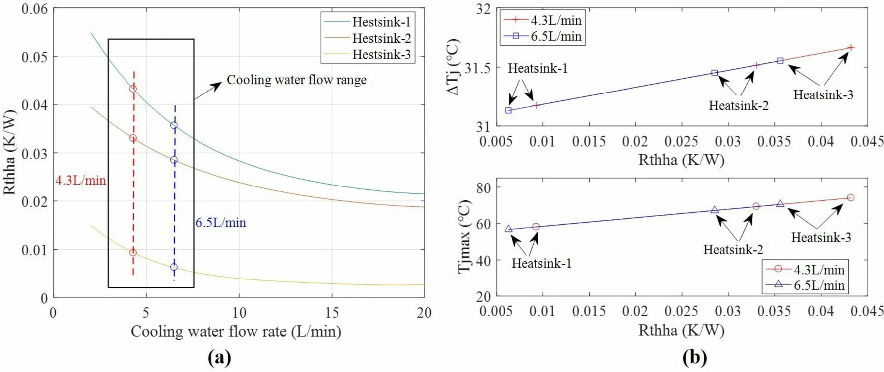
Fig.9 Effects of different parameters on junction temperature fluctuation ΔTj and lifetime Nf.a Thermal resistance of heatsink vs.cooling water flow rate and b fluctuation of ΔTj and maximum Tjmax of junction temperature under different water flow rates and thermal resistances
The fault statistics of power electronic systems show that in addition to semiconductor devices,the reliability of capacitors is crucial.Capacitance plays a role in decreasing the DC-link voltage ripple and balancing the transient power between the front and rear stages of power converters [25]. Capacitance is sensitive to electrical and thermal stresses. Therefore, the reliability of the capacitance needs to be studied further.
6 Conclusion
This paper presented a complete solution for the lifetime estimation of the IGBT module of the accelerator pulsed power supply. Based on power loss discretization, a calculation method for the junction temperature of the accelerator pulsed power supply was presented, and the accuracy and computational complexity were compromised.The test results of the accelerated power cycling test were then fitted to obtain the corrected lifetime model.The junction temperature was verified using an infrared camera,and the error was within 3%. Finally, the lifetime of the IGBT module under the two typical current waveforms was estimated. The flat-top current and switching frequency were found to significantly influence the junction temperature of the IGBT module.The effect of the heatsink on the junction temperature was also discussed.
The proposed method can be applied to other IGBT modules and pulsed power supplies. Moreover, this study provided accurate predictions of the junction temperature and lifetime, as well as assistance for the design of an accelerator pulsed power supply with reduced cost.
Author contributionsAll authors contributed to the study conception and design. Material preparation, data collection, and analysis were performed by Jie Wang, Da-Qing Gao, Wan-Zeng Shen, and Hong-Bin Yan. The first draft of the manuscript was written by Jie Wang and allauthors commented on previous versions of the manuscript. All authors read and approved the final manuscript.
杂志排行

Nuclear Science and Techniques的其它文章
- Thermal hydraulic characteristics of helical coil once-through steam generator under ocean conditions
- Optimization of the cavity beam-position monitor system for the Shanghai soft X-ray free-electron laser user facility
- A beam range monitor based on scintillator and multi-pixel photon counter arrays for heavy ions therapy
- Research on manufacture technology of spherical fuel elements by dry-bag isostatic pressing
- Beam–beam effects and mitigation in a future proton–proton collider
- Ultrahigh accelerating gradient and quality factor of CEPC 650 MHz superconducting radio-frequency cavity