Receding-Horizon Trajectory Planning for Under-Actuated Autonomous Vehicles Based on Collaborative Neurodynamic Optimization
2022-10-29JiasenWangJunWangandQingLongHan
Jiasen Wang,, Jun Wang,, and Qing-Long Han,
Abstract—This paper addresses a major issue in planning the trajectories of under-actuated autonomous vehicles based on neurodynamic optimization. A receding-horizon vehicle trajectory planning task is formulated as a sequential global optimization problem with weighted quadratic navigation functions and obstacle avoidance constraints based on given vehicle goal configurations. The feasibility of the formulated optimization problem is guaranteed under derived conditions. The optimization problem is sequentially solved via collaborative neurodynamic optimization in a neurodynamics-driven trajectory planning method/procedure. Simulation results with under-actuated unmanned wheeled vehicles and autonomous surface vehicles are elaborated to substantiate the efficacy of the neurodynamics-driven trajectory planning method.
I. INTRODUCTION
AUTONOMOUS vehicles are of critical importance for many applications [1], [2] such as cooperative tracking[3], surveillance [4], search and rescue [5], parcel delivery [6],environment monitoring [7], environment exploration [8], adhoc communication [9], [10], land and marine transport[11]–[13], etc. Typical vehicles include unmanned wheeled vehicles (UWVs) [14]–[16], autonomous surface vehicles(ASVs) [17]–[20], unmanned marine vehicles (UMVs) [21],[22], and autonomous underwater vehicles (AUVs) [23]–[25].Motion planning is a fundamental module for task completion by using autonomous vehicles [26]–[31].
Under-actuated vehicles refer to vehicles with fewer actuators than their degrees of freedom. Most land and marine vehicles are under-actuated. Trajectory planning for autonomous vehicles is to plan vehicle motion trajectories from their start configurations to goal configurations, after task assignment[26], [27], [32]. Trajectory planning of under-actuated vehicles is difficult due to their highly limited feasible trajectory spaces. In addition, under-actuated vehicles are vulnerable to obstacle collisions because they cannot be controlled to move in every degree of freedom.
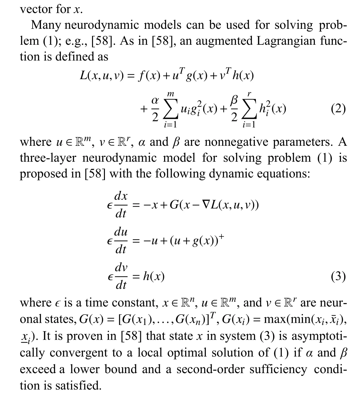
Navigation functions (NFs) are widely used for vehicle navigation planing. For example, differentiable navigation functions are developed for robot navigation [33]. Based on the NFs in [33], an exact method for robot trajectory planning is developed [34]. Extensions of NFs in [33], [34] are available for vehicle trajectory planning [35]–[39]. For example, an NF with heading directions of vehicles is used for trajectory planning of nonholonomic wheeled vehicles, and the closed-loop navigation system is proven to be asymptotically stable [37].Another NF is developed for vehicle trajectory planning in unknown environments [39]. In addition to continuously differentiable NFs, piecewise differentiable NFs are also available for trajectory planning; e.g., [26], [40].
Besides NF-based approaches, several other approaches are also available; e.g., rule-based methods [4], optimization methods [41]–[44], search methods [45], learning methods[46], information fusion methods [47], [48], and their combinations [43], [48]. For example, a bio-inspired trajectory planning method is proposed for under-actuated vehicles working in maze environments [4]. A Hamilton-Jacobi optimization method is used for the trajectory planning of under-actuated drifters in river environments [41]. Evolutionary optimization and fuzzy control methods are used for the trajectory planning of two cooperative mobile robots [42]. A fine-to-coarse search algorithm is developed for robots trajectory planning in regionalized environments [45]. Recently, an NF based on one-dimensional NFs is used in model predictive control for vehicle trajectory planning in static and dynamic environments [43]. A reinforcement learning trajectory planning method is developed based on neural networks and grid representations [46]. A model predictive control algorithm is proposed for long-distance autonomous underwater vehicle trajectory planning based on the declination and inclination components of the geomagnetic field and convex quadratic programming [44]. A service vehicle is navigated based on a robust kinematic control law and data from multiple sensors[47]. A navigation method is presented in [48] based on a brain-machine interface with electroencephalograph (EEG)signals.
Receding-horizon trajectory planning is carried out by sequentially solving optimization problems with an NF and collision-avoidance constraints in a forward-moving window(finite-time horizon). Several receding-horizon vehicle trajectory planning methods are developed [27], [40], [43], [44],[49]–[53]. Specifically, receding-horizon trajectory planning methods are proposed for mobile robots based on an utility function and admissible velocity constraints [49], for unicycles based on piecewise differentiable NFs [40], for mobile robots based on randomized optimization [50], for mobile vehicles based on passivity and continuously differentiable NFs [51], for mobile vehicles via sampling-parametrization[52], for unmanned aerial vehicles via sequential convex optimization [27], for high-speed ground vehicles based on optimization of references [53], for autonomous vehicles based on convex optimization [43], and for AUVs based on quadratic programming [44]. In [40], [51], [52], discrete sampling optimization (DSO) is used for approximately solving optimization problems. Because of the approximation nature, the planned trajectories by using DSO may violate velocity or input constraints [40].
Neurodynamic approaches are also applied for trajectory planning. For example, a competitive neural network for trajectory planning of a nonholonomic mobile robot is developed [54], where the neural network is used to generate robotic trajectory. In addition to neurodynamics-driven trajectory planning, neurodynamic approaches are also applied for model predictive control [55], robust pole assignment [56],velocity estimation [57], command optimization [24], and vehicle task assignments [32], etc.
Although neurodynamic optimization appears in some applications, it has not yet been used for the receding-horizon planning of under-actuated vehicles. It is interesting and meaningful to analyze global convergences of such a planning approach in the presence of kinetics, kinematics, and collision-avoidance constraints.
In this paper, a neurodynamics-driven receding-horizon trajectory planning method is presented for under-actuated vehicles. The receding-horizon trajectory planning is formulated as a sequential global optimization problem, and solved by using collaborative neurodynamic optimization. The contributions of the paper are twofold: 1) The receding-horizon trajectory planning of under-actuated vehicles is formulated as a sequential optimization problem with kinetic, kinematic, collision-avoidance constraints. Conditions are derived for ensuring the feasibility of the sequential optimization problem. 2)The formulated problem is solved via collaborative neurodynamic optimization and conditions are derived for the global convergence of the neurodynamics-driven trajectory planning method.
The differences of the proposed method and existing methods are multifaceted. For example, both kinematics and kinetics are considered herein, whereas kinetics is not considered in[4], [35], [37], [47]. Vehicle kinetics models the dynamic capability of vehicles in motion. Trajectory planning without considering kinetics would often result in the infeasibility of planned trajectories for given vehicles. That is, trajectory planning with both kinetic and kinematic constraints is more practical. A backstepping-based nonsmooth planning and control method in [36] is applicable for navigating unicycle mobile robots with both kinematics and kinetics, it may not be applied to other vehicles such as under-actuated ASVs. In addition, terminal kinematic chattering behaviors [36], [40]are avoided herein via terminal optimization. Moreover, different from the receding-horizon planning approach in [51],no operation with singularity is used herein, and the objective functions are, rather than assumed to be, continuously differentiable. At last, unlike the Lyapunov-based navigation approach in [37] and receding-horizon navigation approach in[50], the neurodynamics-driven method herein is globally convergent rather than locally convergent.
The rest of the paper is organized as follows. Preliminaries are provided in Section II. The neurodynamics-driven trajectory planning method is described in Section III. Specific paradigms on UWVs and ASVs are discussed in Section IV.Simulation results on UWVs and ASVs are elaborated in Section V. Conclusions are given in Section VI.
II. PRELIMINARIES
This section provides necessary background knowledge to facilitate understanding the results in subsequent sections.
A. Navigation Functions

B. Collaborative Neurodynamic Optimization
Consider a general constrained optimization problem

Collaborative neurodynamic optimization (CNO) proposed in [59] is a hybrid intelligent framework for global optimization by employing multiple neurodynamic models for scatter local search and meta-heuristics (e.g., particle swarm optimization) for initial state updating. CNO is proven to be almost surely convergent to the global optima of global optimization problems [59].
III. RECEDING-HORIZON TRAJECTORY PLANNING
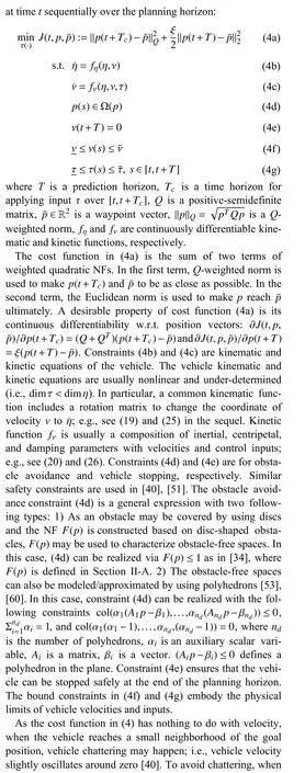
A. Problem Formulation


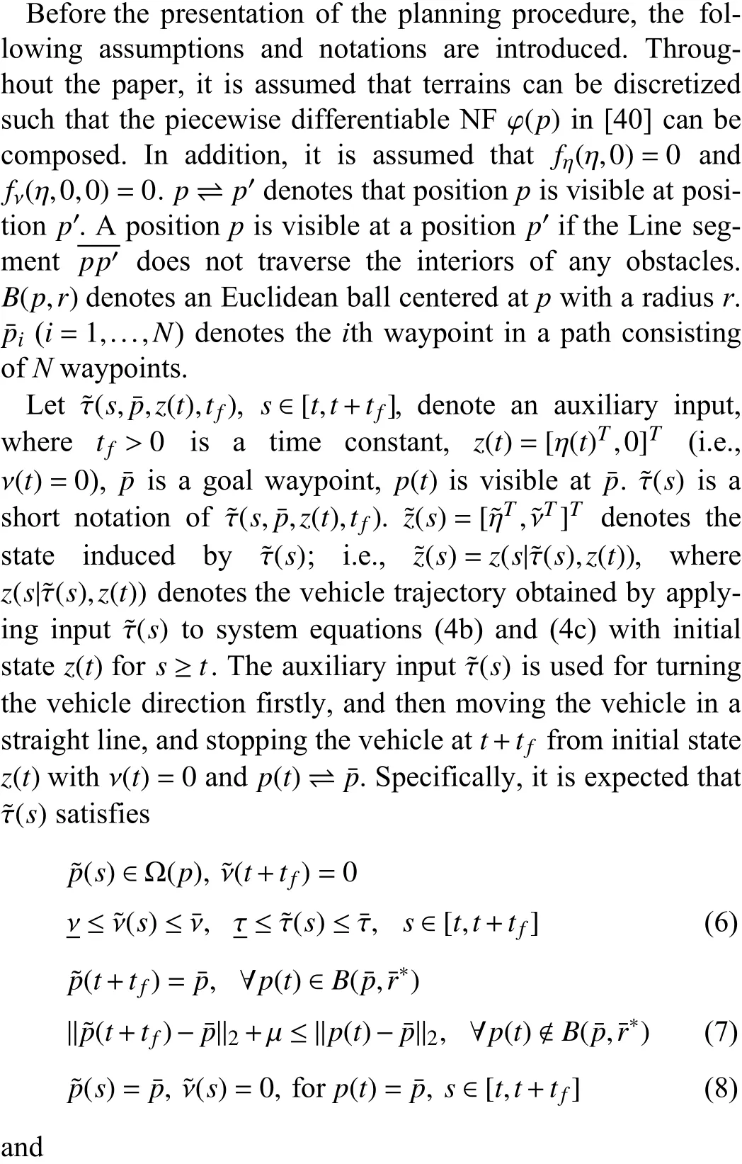
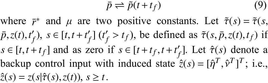
B. Planning Procedure

Procedure 1 Trajectory Planning Procedure 1 Set current goal waypoint index , current time instant ,initial state , , ; Set for such that , , is visible at ,, and is visible at for ; Set for such that ; Set values for T,( ), ξ, Q, P, R, ; ; , ,;t <Tp p(t)∈B(¯pN,rN) ¯pN ⇌ˆp(t+δT)i=1 t=0 ν(0)=0 η(0)=[p(0)T,ψ(0)]T z(0)=[η(0)T,ν(0)T]T ¯pj j=1,...,N φ(¯p j)>φ(¯p j+1) ¯pN =pd ¯p1 p(0)φ(p(0))>φ(¯p1) ¯pj+1 ¯pj 1 ≤j ≤N-1 r j >0 j=1,...,N B(¯p j,rj)∩B(¯pk,rk)=Ø, ∀j ≠k Tc T ≥Tc Tp δT =T-Tc ˆτ(s)=0 ˆz(s)=z(s|ˆτ(s),z(0))s ∈[0,δT]2 while but not ( and ) do τ*(s) s ∈[t,t+T]J(t,p,¯pi)3 Obtain for by solving problem (4) with cost function using CNO;z*(s)=z(s|τ*(s),z(t)) s ∈[t,t+T]4 for ;¯pi ⇌p*(t+T) ˆp(t+δT)≠¯pi 5 if and then τ(s)=τ*(s) z(s)=z*(s) s ∈[t,t+Tc]6 , for ;ˆτ(s)=τ*(s) ˆz(s)=z(s|ˆτ(s),z(t)) s ∈[t,t+T]7 , for ;8 ;9 else¯pi ⇌ˆp(t+δT)t=t+Tc 10 if then ˆτ(s)= ˜τ(s,¯pi,ˆz(t+δT),Tc) s ∈(t+δT,t+T]11 for ;12 else ˆτ(s)= ˜τ(s,¯pi-1,ˆz(t+δT),Tc) s ∈(t+δT,t+T]13 for ;14 end ˆz(s)=z(s|ˆτ(s),ˆz(t+δT)) s ∈(t+δT,t+T]15 for ;τ(s)= ˆτ(s) z(s)=ˆz(s) s ∈[t,t+Tc]16 , for ;t=t+Tc 17 ;18 end¯pi ⇌ˆp(t+δT) p(t)∈B(¯pi,ri) 1 ≤i ≤N-1 19 if , , and then i=i+1 20 ;21 end 22 end t <Tp 23 while do τ*(s) s ∈[t,t+T]24 Obtain for by solving problem (5) using CNO;τ(s)=τ*(s) z(s)=z*(s) s ∈[t,t+Tc]25 , for ;26 ;27 end t=t+Tc
The procedure of the neurodynamics-driven trajectory planning approach is detailed in Procedure 1. Line 1 is to initialize states, waypoints, radii, problem parameters, etc. In particular,iis an index for the current waypoint and initialized as one; i.e., the first waypoint. It ends with valueN; i.e., the goal position. The current timetindicates that the current planning horizon is . Lines 2-21 are steps in a while loop for driving the vehicle from the initial position to the neighborhood of . In Line 2, the while loop runs if the visibility or proximity condition is not verified. In Lines 3 and 4, and for are obtained by using the solution of problem (4). In Lines 6 and 7, the planned control input , planned trajectory , backup control input ,and backup trajectory are updated by using and[t,t+T]p(0)B(pd,rN)pdτ*(s)z*(s)s∈[t,t+T]τ(s)z(s) ˆτ(s)ˆz(s) τ*(s)z*(s)Tcto the next planning horizon. In Lines 11, 13, and 15, the backup control and trajectory are updated by using the auxiliary control to ensure visibility. In Line 16, the planned control and trajectory are updated by using the backup control input and trajectory to ensure visibility. In Line 17,tis increased byTcfor moving to the next planning horizon. In Line 20,iis added by one to switch from waypointito waypointi+1 if the visibility and proximity conditions in Line 19 are verified. Lines 23-26 are steps in a while loop for driving vehicle position inB(pd,rN) to the goal positionpdwhile optimizing vehicle velocities. Specifically, Line 24 is to solve terminal problem (5) to obtain solution τ*(s). Line 25 is to update the planned control input and trajectory. Line 26 is to update timettot+Tc.
C. Feasibility and Convergence

quent iterations. Condition 3) requires that the backup velocity is zero at timet+δTfor ensuring safety. Condition 4) is used for ensuring convergence in terms of distance. Condition 5) requires thatTcis lower bounded. Without it, the procedure may not be convergent. Condition 6) requires that there exists an auxiliary control to move the vehicle to the goal waypoint while ensuring visibility. The proof to Lemma 1 is presented as follows.


IV. SPECIFIC PARADIGMS
A. Unmanned Wheeled Vehicles
Consider an UWV with the following kinematic and kinetic equations [14], [55], [63]:


B. Autonomous Surface Vehicles


TABLE I PARAMETER SETUPS

V. SIMULATION RESULTS
A. Settings
Five terrains (a)-(e) are used, where terrains (a)-(d) are benchmarks respectively from [40], [51], [26], and [46],whereas terrain (e) is modified from the terrain in [40]. In this case, constraint (4d) uses multiple rectangles and parallelograms to describe obstacle-free spaces.F(p)≤1 may also be used with increased complexity.
To compute the shortest paths from the initial position to the goal position, the terrains are discretized by using regular grids with an edge length being 0.05 m. Many waypoints along the shortest paths are used. In addition, to ensure waypoints to be far away from obstacles, the obstacles in terrains(a)-(e) are enlarged by 0.25 m, 0.25 m, 0.5 m, 0.5 m, and 0.2 m, respectively. To reduce the number of waypoints, pre-processing is used as follows: Let the goal position be the last waypoint; start from the initial positionAof the vehicle, find a waypointBsuch that the next waypoint ofBbecomes invisible atA; setAtoBand repeat the process until the goal position. By using the processing, preprocessed waypoints and related parameters are listed in Table I.
B. UWV Trajectory Planning

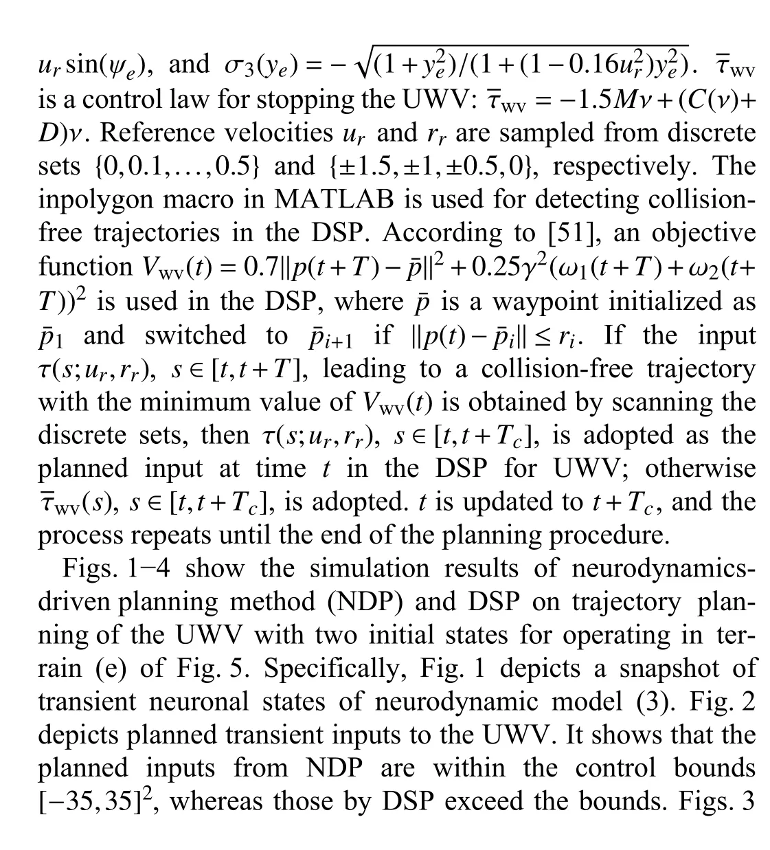

Fig. 1. A snapshot of transient neuronal states of neurodynamic model (3)in the UWV trajectory planning.
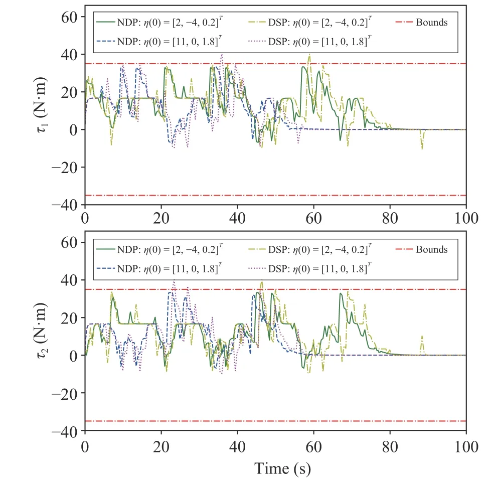
Fig. 2. Planned transient inputs to the UWV with two initial states.

Fig. 3. Planned transient velocities of wheels of the UWV with two initial states.

Fig. 4. Planned transient positions and orientations of the UWV with two initial states.
and 4 depict the planned transient states of the UWV. Fig. 3 shows that the planned velocities using NDP are within the bounds, whereas the ones using DSP exceed the bounds. Fig. 5 depicts planned position trajectories and heading directions of UWVs with two initial states operating in terrains (a)-(e)using the NDP. The results in the figures show that the neuronal states are convergent and the neurodynamics-driven trajectory planning method is able to generate collision-free UWV trajectories in the obstacle-laden terrains.
C. ASV Trajectory Planning


Fig. 5. Planned position trajectories and heading directions of the UWVs with two initial states operating in terrains (a)–(e) using the NDP.

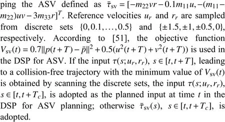

Fig. 6. A snapshot of transient neuronal states of neurodynamic model (3)for ASV trajectory planning.

Fig. 7. Planned transient inputs to the ASV with two initial states.
Figs. 6-9 show the simulation results of neurodynamicsdriven planning method (NDP) and DSP on ASV trajectory planning with two initial states for operating in terrain (d) of Fig. 10. Specifically, Fig. 6 depicts a snapshot of transient neuronal states of neurodynamic model (3). Fig. 7 depicts the planned transient control inputs to the ASV. It shows that the inputs obtained by using NDP are within the bounds, whereas the ones by DSP exceed the bounds. Figs. 8 and 9 depict the planned transient states of the ASV. Fig. 8 shows that velocities planned by NDP are within the bounds, whereas the ones by DSP exceed the bounds. Fig. 10 depicts the planned ASV trajectories and heading directions with two initial states operating in terrains (a)-(e) by using NDP. The results in the figures show that the neurodynamics are convergent and the neurodynamics-driven trajectory planning method is able to generate collision-free ASV trajectories in the obstacle-laden terrains.
VI. CONCLUDING REMARKS
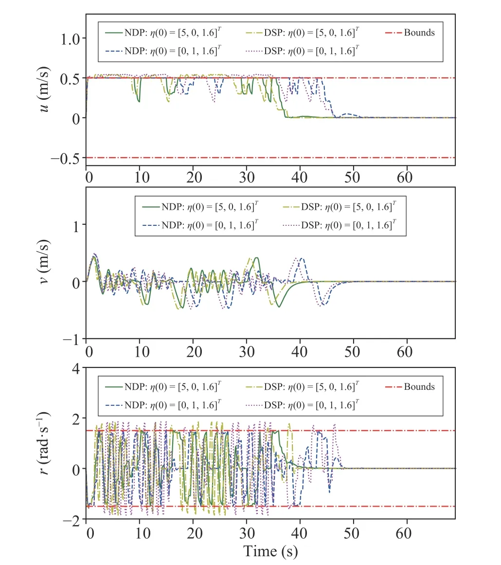
Fig. 8. Planned transient velocities of the ASV with two initial states.

Fig. 9. Planned transient positions and orientations of the ASV with two initial states.
A neurodynamics-driven receding-horizon trajectory planning method is presented for navigating under-actuated vehicles. The proposed trajectory planning method is shown to be convergent to collision-free trajectories, under given assumptions and conditions. Simulation results on under-actuated unmanned wheeled and autonomous surface vehicles substantiate the efficacy of the neurodynamics-driven trajectory planning method. Further investigations may aim at developing new neurodynamics-driven vehicle fleet trajectory planning and tracking control methods based on other obstacle avoidance mechanisms such as artificial potential fields and control barrier functions.

Fig. 10. Planned position trajectories and heading directions of the ASVs with two initial states operating in terrains (a)–(e) by using the NDP.
杂志排行

IEEE/CAA Journal of Automatica Sinica的其它文章
- Adaptive Generalized Eigenvector Estimating Algorithm for Hermitian Matrix Pencil
- Recursive Filtering for Nonlinear Systems With Self-Interferences Over Full-Duplex Relay Networks
- A Zonotopic-Based Watermarking Design to Detect Replay Attacks
- A Bi-population Cooperative Optimization Algorithm Assisted by an Autoencoder for Medium-scale Expensive Problems
- On RNN-Based k-WTA Models With Time-Dependent Inputs
- Frequency Regulation of Power Systems With a Wind Farm by Sliding-Mode-Based Design