Adaptive Generalized Eigenvector Estimating Algorithm for Hermitian Matrix Pencil

Yingbin Gao

Abstract—Generalized eigenvector plays an essential role in the signal processing field. In this paper, we present a novel neural network learning algorithm for estimating the generalized eigenvector of a Hermitian matrix pencil. Differently from some traditional algorithms, which need to select the proper values of learning rates before using, the proposed algorithm does not need a learning rate and is very suitable for real applications. Through analyzing all of the equilibrium points, it is proven that if and only if the weight vector of the neural network is equal to the generalized eigenvector corresponding to the largest generalized eigenvalue of a Hermitian matrix pencil, the proposed algorithm reaches to convergence status. By using the deterministic discretetime (DDT) method, some convergence conditions, which can be satisfied with probability 1, are also obtained to guarantee its convergence. Simulation results show that the proposed algorithm has a fast convergence speed and good numerical stability. The real application demonstrates its effectiveness in tracking the optimal vector of beamforming.

I. INTRODUCTION

THE generalized Hermitian eigenvalue problem (GHEP)has been attracting great attention in many fields of signal processing and data analysis, such as adaptive beamforming [1], wireless communications [2], blind source separation[3], data classification [4] and fault diagnosis [5]. Generally,the GHEP is to find a vectorw∈Rn×1and a scalar λ ∈R such that

whereRy,Rx∈Rn×nare twon×nHermitian and positive definite matrices. The solution vectorwand scalar λ are called the generalized eigenvector and generalized eigenvalue,respectively, of the matrix pencil (Ry,Rx). Traditionally, some numerical algebraic approaches, such as the Jacobi-Davidson and Cholesky factorization, are implemented for the GHEP.However, these approaches are computationally intensive when dealing with higher dimensional input data [6]. Besides,for some scenarios, the sensors can only provide the sampled values of the signals. The matrix pencil is not explicitly given and has to be directly estimated from these sampled values.Hence, it is important to seek a fast and online algorithm for the GHEP adaptively.

Recently, neural network approaches for the GHEP have attracted great attention [7]–[14]. Serving as an online approach, neural algorithm can avoid the computation of the covariance matrix and is suitable for high dimensional input data [15]–[18]. Based on neural network, a variety of learning algorithms for the GHEP have been proposed. For example,the recurrent neural network (RNN) algorithm [19], Yanget al.algorithm [20], canonical correlation analysis (CCA)algorithm [21], adaptive normalized Quasi-Newton (ANQN)algorithm [22] and generalized eigen-pairs extraction (GEPE)algorithm [23] can be used to estimate the first generalized eigenvector, which is defined by the generalized eigenvector corresponding to the largest generalized eigenvalue of the matrix pencil. Conversely, to compute the generalized eigenvector corresponding to the smallest generalized eigenvalue,which is referred to as the last generalized eigenvector hereafter, Nguyenet al.[24] proposed the generalized power (GP)algorithm and Liet al. [25] proposed the generalized Douglas minor (GDM) component analysis algorithm. Due to the fact that the first generalized eigenvector of the matrix pencil(Ry,Rx)is also the last generalized eigenvector of the matrix pencil (Rx,Ry), the above mentioned algorithms are equivalent in practice. For these algorithms, the convergence performance heavily lies on the learning rate: too small a value will lead to slow convergence and too large a value will lead to oscillation or divergence [21]. Hence, how to select the right learning rate becomes an important issue before using these algorithms.

Generally, the neural network algorithm is described by its stochastic discrete-time (SDT) system, and it is a difficult task to directly study the SDT system when analyzing the convergence properties of these algorithms. In order to solve this problem, some indirect analysis methods have been proposed,such as the ordinary differential equations (ODE) method[19], the deterministic continuous-time (DCT) method [26]and the deterministic discrete-time (DDT) method [27].Among these methods, the DDT method is the most reasonable analysis approach since it can preserve the discrete-time nature of the original algorithms and provide some conditions to guarantee their convergence [28]. Due to these advantages,the DDT method has been widely used to analyze the neural network algorithms [24], [25], [29]–[33]. Unfortunately, the convergence conditions obtained in the above literatures are all related to the learning rate. For example, for the ANQN algorithm and the GDM algorithm, the learning rate should satisfy μ ＜2λn/(λ1-λn) and μ ＜0.2/λ1, respectively. Herein,λ1and λnare the largest and smallest generalized eigenvalues,respectively, of the matrix pencil (Ry,Rx). These convergence conditions are not suitable for real practice. Firstly, the range of learning rate is usually given by 0 ＜μ ≤1, and the value regions are greatly reduced by these restricted conditions. Secondly, in many cases, the generalized eigenvalues are unknown in advance, so it is difficult to choose the learning rate according to these convergence conditions.

From the above analysis, the learning rate seems to be very important for both algorithms developing and their convergence analysis. However, is the learning rate an indispensable part for neural network algorithms? In this paper, in order to eliminate the effect of the learning rate, we propose a novel neural network algorithm for the GHEP. Differently from the previous algorithms, the proposed algorithm does not need a learning rate. Hence, the issue to select its value is avoided.Traditionally, during the process of analyzing the convergence properties via the DDT method, some restrictions are added to the learning rate in order to guarantee the establishment of some inequalities, which are necessary for the process of proof. However, since the learning rate has been removed, the analysis process of the proposed algorithm will also be quite different from those of the previous algorithms.Herein, we will try to analyze the proposed algorithm by using the DDT method in another way and derive some convergence conditions.

The main contributions of this paper are summarized as follows. 1) To estimate the first generalized eigenvector, a novel algorithm is proposed when the matrix pencil is explicitly provided. 2) To prove the convergence result of the proposed algorithm, the fixed stability of the proposed algorithm is analyzed by the Lyapunov function approach. 3) The convergence analysis is accomplished by the DDT method and some convergence conditions are also obtained. 4) An online adaptive algorithm is derived when the generalized eigenvector is needed to be calculated directly from the input signal or data sequences.

The remainder of this paper is organized as follows. Section II formulates the novel neural network algorithm for the GHEP.Section III investigates the properties of the equilibrium points. Section IV provides the online version of the proposed algorithm. Section V analyzes the convergence property of the proposed algorithm via the DDT method. Section VI presents some numerical simulation results to illustrate the effectiveness of the proposed algorithm. Section VII applies the proposed algorithm to solve the real problem of adaptive beamforming. Section VIII concludes this paper.

II. PRELIMINARIES AND NOVEL LEARNING ALGORITHM

A. Notations

In order to have a better understanding of the symbols used throughout this paper, some essential notations are listed as follows.

R: The autocorrelation matrix of input signal;

x,y: The input signals;

v: The generalized eigenvector;

I: The identity matrix;

w: The weight vector of neural network;

z: The projection length ofwontov;

λ: The generalized eigenvalue;

δij: The Kronecker delta function;

α: Forgetting factor.

B. Generalized Eigen-Decomposition

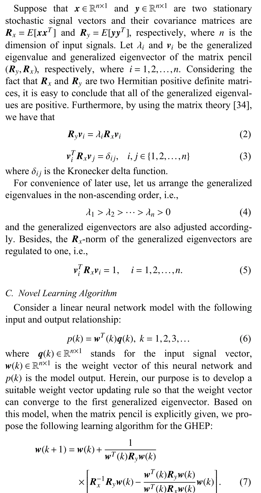
Traditionally, the learning rate is usually added before the square brackets to adjust the step size of the neural network algorithms. However, the learning rate does not appear in (7).Through comparing the structure of the proposed algorithm with those of some existing algorithms, the GDM algorithm for example [25], it seems that the learning rate is changed into the term 1 /[wT(k)Ryw(k)]. However, this equation is actually very different from the learning rate. The value range of the learning rate is 0 ＜μ ≤1, however, the term 1/[wT(k)Ryw(k)]has much wider value range because of the randomicity of the weight vectorw(k).

For the proposed algorithm, we are interested in its equilibrium points. Specifically, we consider the following two questions.

1) Does this algorithm have the ability to converge to the first generalized eigenvector?

2) Does this algorithm have the unique convergence status?

The above two questions mainly concern the finial convergence result of the proposed algorithm, and their answers will be given in the next section.

III. STABILITY OF THE EQUILIBRIUM POINTS

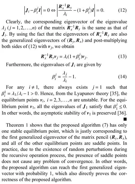
Before answering the above two questions, let us firstly seek out all the equilibrium points of the proposed algorithm.Denote the following matrix function:

IV. ONLINE VERSION OF THE PROPOSED ALGORITHM

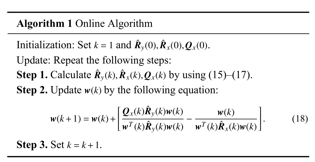
Algorithm 1 Online Algorithm k=1 ˆRy(0), ˆRx(0),Qx(0)Initialization: Set and .Update: Repeat the following steps:ˆRy(k), ˆRx(k),Qx(k)Step 1. Calculate by using (15)–(17).Step 2. Update by the following equation:w(k)w(k+1)=w(k)+■■■■■■Qx(k)ˆRy(k)w(k)wT(k)ˆRy(k)w(k)- w(k)wT(k)ˆRx(k)w(k)■■■■■■. (18)Step 3. Set .k=k+1

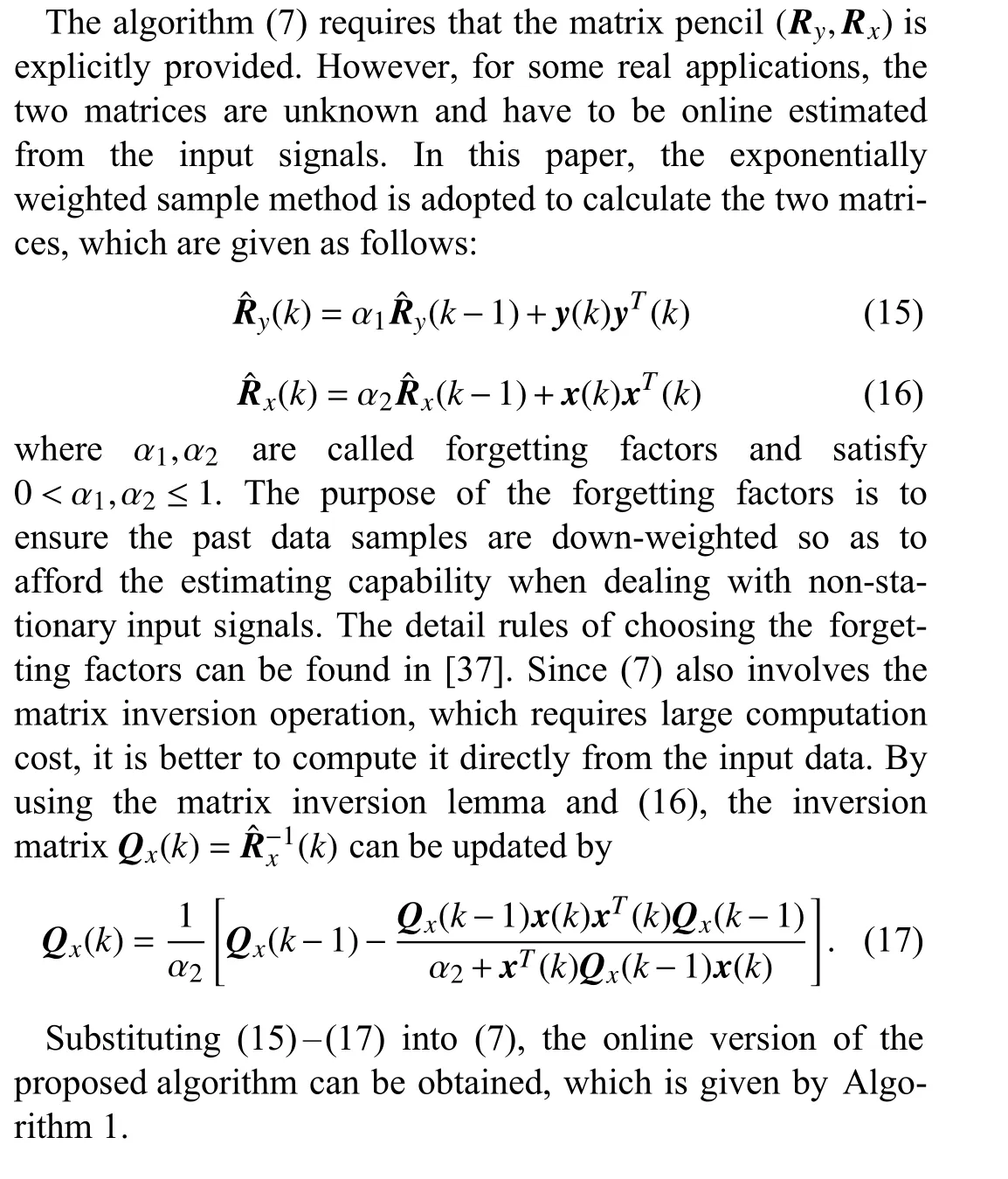
Although (18) and (7) are two different forms of the proposed algorithm, they are suitable for different cases. The online algorithm (18) is suitable for the scenario where the sensors can only provide the sampled values of the signals rather than the autocorrelation matrices. However, (7) needs that the matrix pencil is explicitly given.

Next, we discuss the full computational complexity of the online algorithm. For clarity, the computation cost of each term is summarized in Table I. As a result, the online algorithm needs 1 0n2+6nmultiplications per updating, which has the same magnitude as the existing algorithms [24], [25].

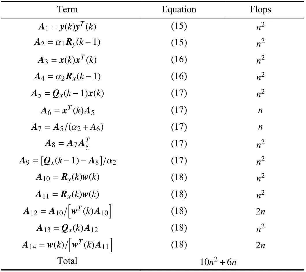
TABLE I COMPUTATIONAL COMPLEXITY

V. CONVERGENCE CHARACTERISTIC ANALYSIS

A. Analysis Preliminary

In this section, we investigate the convergence characteristic of the proposed algorithm via the DDT method. Through adding the condition expectation to (18) and identifying the expected value as the next iteration, the DDT system of the online algorithm is obtained, which is justly equivalent to (7).That is to say, (7) can also be seen as the average version of the online algorithm and can describe the average dynamical behavior of the online algorithm (18).

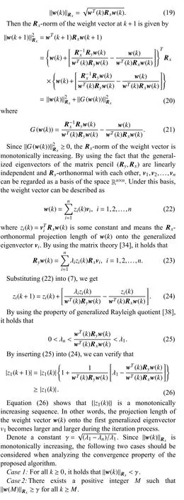
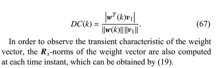
Prior to analysis, let us provide some preliminaries. Denote theRx-norm of the weight vector at the time instantkby

B. Convergence Analysis in Case 1

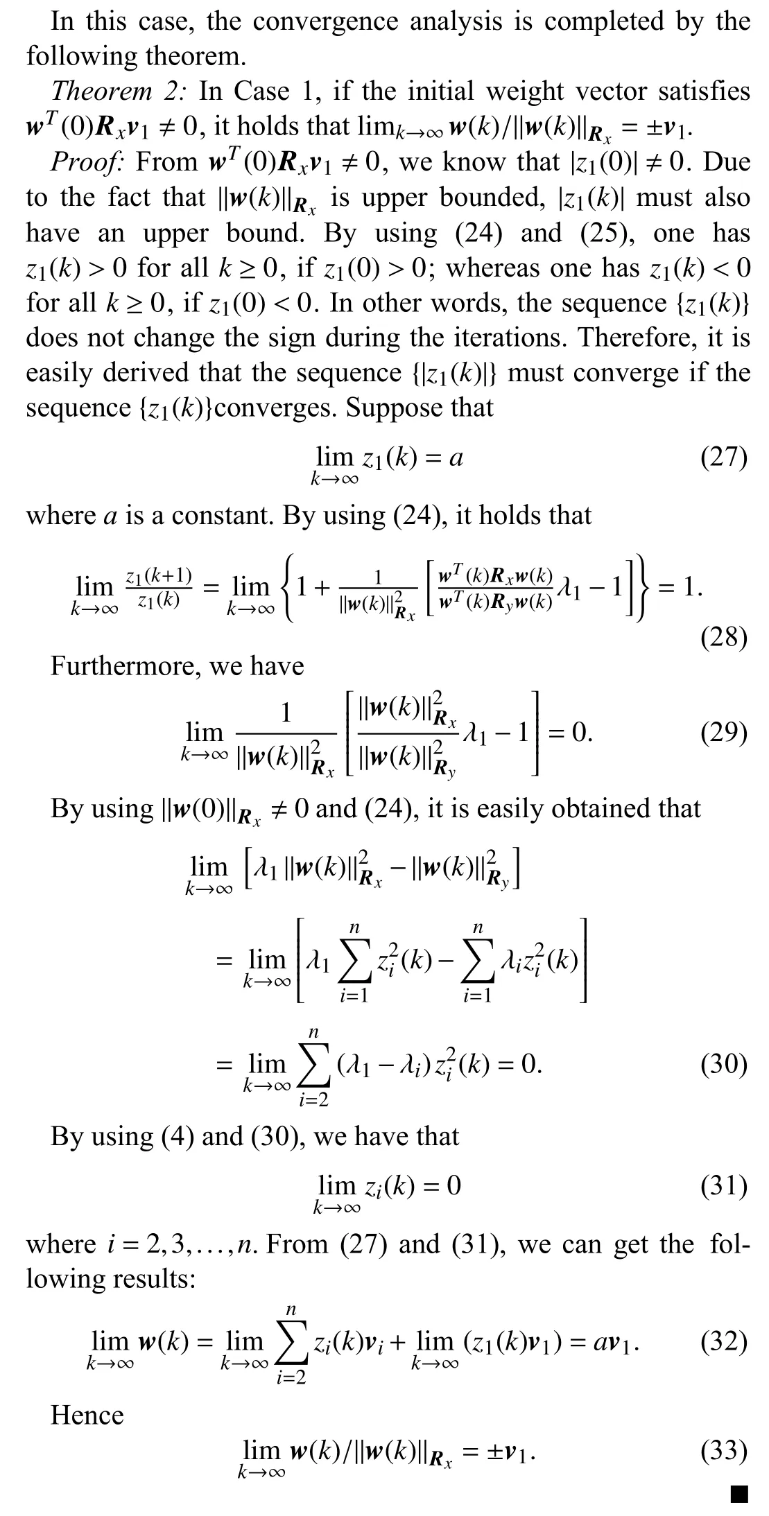
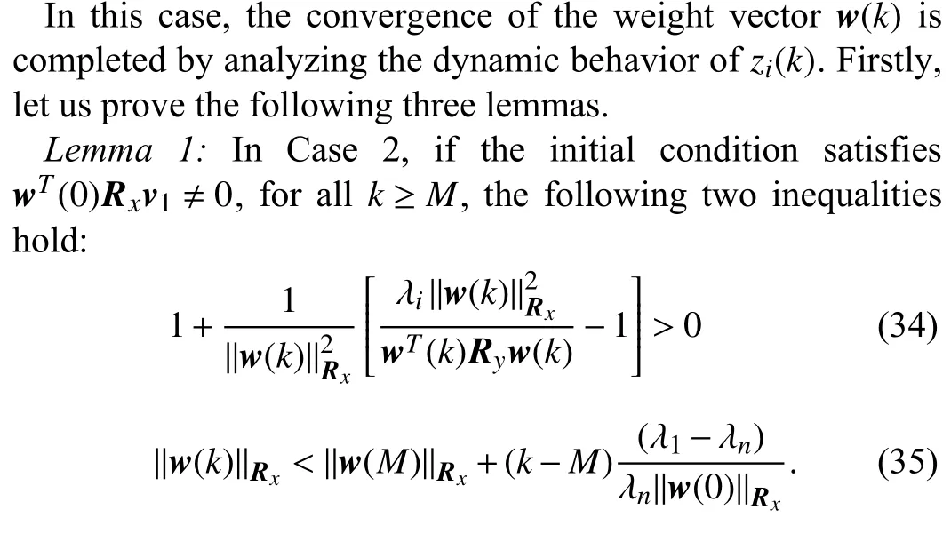
C. Convergence Analysis in Case 2

D. Analysis Conclusions and Remarks

Through comparing the results of Theorems 2 and 3, it is easy to conclude that the convergence results have no relationship with the two cases. And γ is only used to divide the two cases, and its value is selected in order to complete the proof.So combining the two theorems, the final analysis conclusion is obtained.

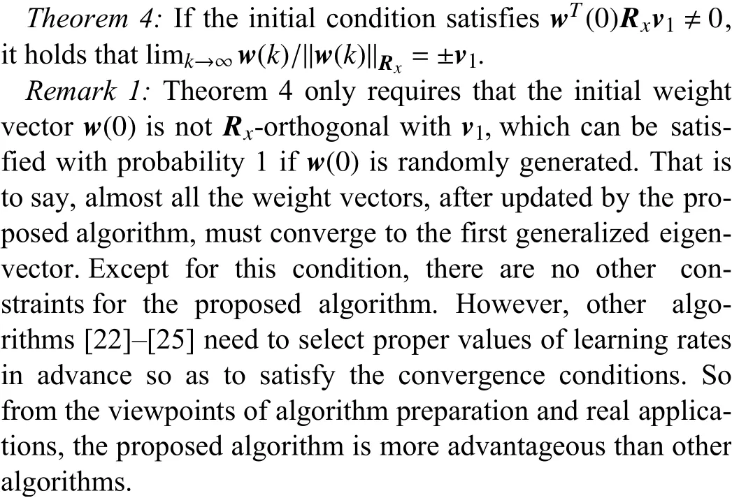
Remark 2:The proposed algorithm is suitable for estimating the first generalized eigenvector of a matrix pencil. To track the generalized subspace spanned by several generalized eigenvectors, the nested orthogonal complement structure method in [24] can be used. When the multiple generalized eigenvectors are needed, the sequential extraction method in [25] can be adopted. Since the two methods are mature technologies and can be easily transplanted into the proposed algorithm, we do not discuss them in this paper, and interesting readers may refer to them for details.

VI. NUMERICAL SIMULATIONS

This section provides three simulation experiments to show the performance of the proposed algorithm. The first experiment aims to extract the first generalized eigenvector of a matrix pencil and compares the results with some existing algorithms. The second experiment serves to directly estimate the first generalized eigenvector from two input signals. The third experiment is designed to verify the correctness of the analysis conclusions obtained in Section V.

A. Contrast Experiment

In this part, the proposed algorithm, RNN algorithm [19],ANQN algorithm [22] and GEPE algorithm [12] are implemented to estimate the first generalized eigenvector of the matrix pencil (Ry,Rx) composed by the following two6×6 positive definite matrices, which are randomly generated by using the method in [28]

The DC and norm curves of these algorithms are shown in Figs. 1 and 2, respectively. In Fig. 1, it is obvious that all of the DC curves converge to unit one, which means that these algorithms, including the proposed algorithm, have reached to the direction of the first generalized eigenvector. Among these algorithms, the proposed algorithm has the fastest convergence speed. From Fig. 2, we can see that all the norm curves of these algorithms reach to the convergence status at last.However, the convergence values are not the same. For the proposed algorithm, GDM algorithm and GEPE algorithm, the weight vector norms always increase at the beginning and then reaches a fixed value. Clearly, for the proposed algorithm, the dynamic behavior of the weight vector norm is consistent with the theoretical theory analysis in Section V. For the RNN algorithm and GDM algorithm, the norms gradually decrease to the final value. Due to the existence of normalization operation, the weight vector norms of the GP algorithm and ANQN algorithm are equal to unit one during all the iterations. Except for the GP algorithm and the ANQN algorithm,the weight vector norm of the proposed algorithm converges faster than those of the other three algorithms.

Fig. 1. Direction cosine curves of these algorithms.

B. Online Extraction

In this experiment, the proposed algorithm is used to estimate the first generalized eigenvector directly from the input signals. The results are also compared with those obtained by the RNN algorithm [19], ANQN algorithm [22], GEPE algorithm [12], GP algorithm [24] and GDM algorithm [25]. Consider the following two equations:algorithm and μ=0.005 for the RNN algorithm. Clearly, all the convergence conditions can be satisfied through these settings. Besides, we set λ (0)=100 for the ANQN algorithm. All of these algorithms are tested throughT=100 independent runs.

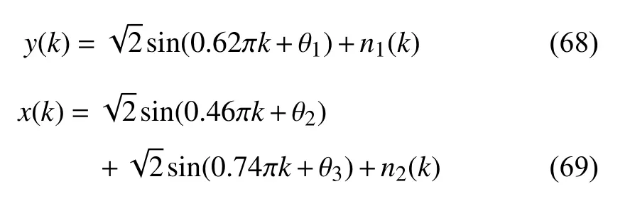
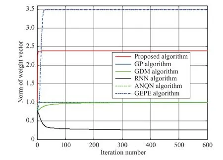
Fig. 2. Norm curves of these algorithms.

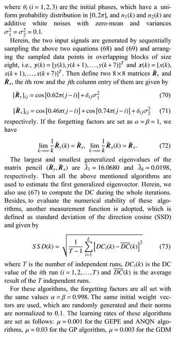
Figs. 3 and 4 provide the average DC and SSD curves of these algorithms, respectively. From Fig. 3, we can see that the DC curve of the proposed algorithm converges to unit one after about 1000 iterations, which means that the proposed algorithm can directly extract the first generalized eigenvector from the input signals. When compared with other algorithms, the proposed algorithm shows the fastest convergence speed. In Fig. 4, the simulation results of the last 4000 iterations are shown separately by a small figure. From this figure,we observe that the final SSD value of the proposed algorithm is less than those of other algorithms, which means that the proposed algorithm has the best numerical stability among these algorithms.

Fig. 3. DC curves for online extraction.

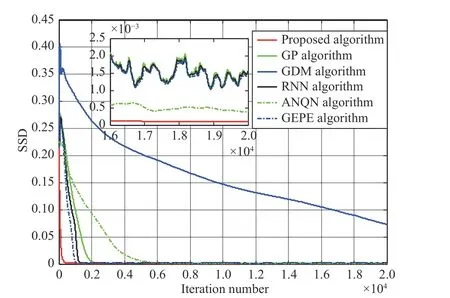
Fig. 4. SSD curves for online extraction.

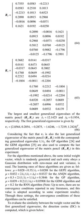
C. Convergence Experiment

In this experiment, we also use the proposed algorithm to compute the first generalized eigenvector of the matrix pencil composed by (64) and (65). Since the tracking ability has been proven in the above two experiments, we concern other two evaluated functions in this experiment. The first one is the

Same as the above experiments, the initial weight vector is also randomly generated. Figs. 5 and 6 show the simulation results when the following initial weight vector is adopted.

Fig. 5. Projection length curves.

VII. ADAPTIVE BEAMFORMING

Recently, array signal processing has been widely used in the area of wireless communication systems. In cellular mobile communication, with the increment of the communication channels, it is essential to improve the frequency spectrum reuse technique (FSRT). Adaptive beamforming, which is also called spatial filtering, is an integral part of FSRT and has attracted much more attention [39]–[53]. Through weighted summing the measured signals observed by an array of antennas, the spatial filter can form a directional beam,which ultimately leads to the maximum expected signal and the minimization of noises from the environment and interferences from other subscribers. If the weights in the antennas can be automatically adjusted with the signal environment, it is called adaptive beamforming [54].

Let us consider the scenario where the impinging signals are narrowband. Fig. 7 provides an example of a uniform linear array, which hasnantenna elements with half-wavelength spacing. The amplitude and phase of the impinging signal in each channel are adjusted by a weighted coefficientwi(k),i=1,2,...,n, and the array output is given by

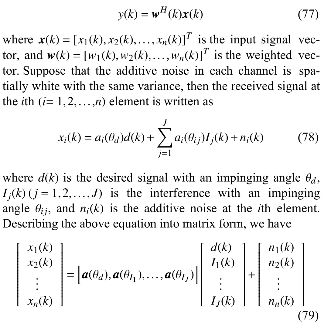
Fig. 6. Entries of w¯.

and

Fig. 7. Narrowband beamformer.

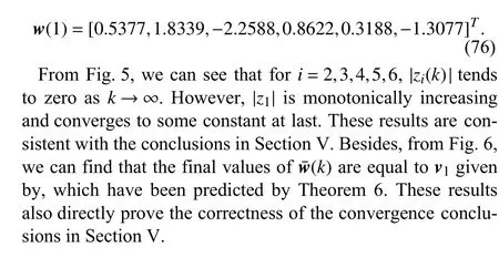
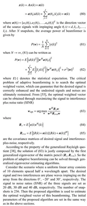
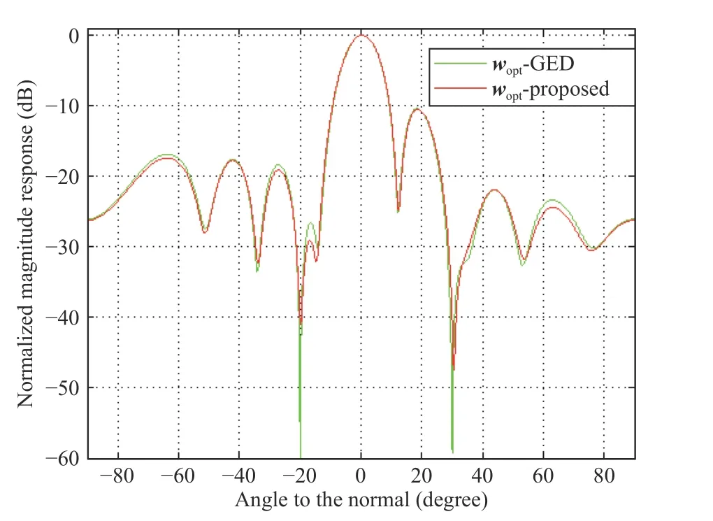
Fig. 8. Beam pattern.

Fig. 8 shows the simulation results obtained by the proposed algorithm and batch method (i.e., the exact values of the first generalized eigenvector), which are marked with the red line and green line, respectively. From this figure, we can see that the main beamforming has a strong main lobe around the desired signal and the interferences are greatly suppressed.Besides, the results of the proposed algorithm are similar with those of the batch method, which means the proposed algorithm has good performance of tracking the optimal beamforming vector.

VIII. CONCLUSION

In this paper, we devoted to eliminating the affection of learning rate for neural network algorithms and proposed a novel algorithm without learning rate, which can be used to estimate the first generalized eigenvector of a matrix pencil.The stability and the convergence characteristic of the proposed algorithm are also analyzed by using the Lyapunov method and the DDT method, respectively. Numerical simulations and real applications were carried out to show the performance of the proposed algorithm. Since the operations in the proposed algorithm are simple matrix addition and multiplications, it is easy for the systolic array implementation.

As a future research direction, we may focus on how to reduce the computation complexity and develop new fast and stable algorithms without learning rate. Since there are so many algorithms reported in literatures, an interesting idea is to build a general framework, which can remove the learning rates in these algorithms. Besides, improving algorithm’s robustness is also important. We plan to address these issues in the future.