A Solution Method for a Mixed Stochastic Linear Second-order Cone Complementarity Problem
2022-09-06WANGGuoxinLIUYanjuanHUXiaoli
WANG Guoxin, LIU Yanjuan, HU Xiaoli
(School of Mathematics and Physics, Nanyang Institute of Technology, Nanyang Henan 473004, China)
Abstract: Due to the fact that the stochastic problems usually do not exist a solution suitable to all realizations, the paper employs the expected residual minimization (ERM) formulation to solve the mixed stochastic linear second-order cone complementarity problem. The Monte Carlo method is employed to approximate the ERM problem. The coercivity of the ERM problem and the approximation problem is discussed, and the convergence of the approximation problem is also given. Furthermore, the theoretical results are applied to a stochastic optimal power flow with radial network structure in power system and some numerical experiments are given for the real-world Southern California Edison 47-bus network.
Key words: mixed stochastic linear second-order cone complementarity problem; expected residual minimization; Monte Carlo method; stochastic optimal power flow
1 Introduction
Consider the following mixed stochastic linear second-order cone complementarity problem: find a vectorx∈nsuch that
x∈K,M(ω)x+q(ω)∈K,xT(M(ω)x+q(ω))=0,F(x,ω)=0, a.e.ω∈Ω,
(1)
whereK∶=Kn1×Kn2×…×Knlis a second-order cone withn1+n2+…+nl=nand
Kni∶={(x1,x2)∈×ni-1|x1≥‖x2‖},i=1,2,…,l,
‖·‖ stands for the Euclidean norm,Ωdenotes the support set of the random variableω, “a.e.” is the abbreviation for “almost every” under the underlying probability measure,M(ω)∈n×nandq(ω)∈nfor eachω∈Ω, andF∶n×Ω→nis twice continuously differentiable with respect toxand continuous with respect toω. For simplicity of discussion, we assume that the support setΩis a nonempty and compact set in a finite dimensional Euclidean space.
IfΩcontains only one realization, the problem (1) reduces to the mixed linear second-order cone complementarity problem
x∈K,Mx+q∈K,xT(Mx+q)=0,F(x)=0,
(2)
which has been studied by Egging(2013)[1], Chen and Pan(2012)[2], Fukushima et al.(2002)[3], and Narushima et al.(2013)[4]and the references therein. However, in many practical cases, there may be uncertain parameters in problem (2), which raises the problem (1). In problem (1), the support setΩof a probability distribution is the closure of a set containing all possible values of uncertain variableω, and the probability distribution may be Gaussian distribution, Poisson distribution, uniform distribution and so on. In general, due to the existence of random variables, the problem (1) may not have a common solution that is applicable to all realizable cases. Therefore, a feasible method in dealing with these stochastic problems is to construct a deterministic model that yields a reasonable approximation for uncertain situations.
2 Preliminaries
In this paper, motivated by the work (Chen and Fukushima(2005)[5]), we use the expected residual minimization (ERM) method to solve problem (1). In order to use this method, we need to introduce the so-called second-order cone complementarity functionφ∶n×n→n, which satisfies
φ(x,y)=0 ⇔x∈K,y∈K,xTy=0.
Among the various second-order cone complementarity functions given for linear second-order cone complementarity problems in the literature, we consider the parametric SOC complementarity function
withτ∈(0,4) to be a fixed parameter, wherex∘ydenotes the Jordan product ofxandy, which is defined asx∘y∶=(xTy,x1y2+y1x2) withx=(x1,x2) andy=(y1,y2)∈×n-1, andx2denotes the Jordan product ofxand itself,withx∈Kis the unique square root ofxsuch thatx≠0, see Faraut and Koranyi(1994)[6]for more details about the Jordan product associated with symmetric cones. The functionφτis proposed by Chen and Pan(2010)[7]and the globally Lipschitz continuity and strong semismoothness ofφτhave been shown in Pan and Chen(2010)[8].
By employing the functionφτ, the problem (1) can be transformed equivalently into the stochastic equations
Φ(x,ω)=0,F(x,ω)=0, a.e.ω∈Ω,
whereΦ(x,ω)∶=φτ(x,M(ω)x+q(ω)). Then the ERM formulation for (1) is
(3)
whereEdenotes the expectation operator.
Notice that the objective function of the ERM problem (3) contains an expectation, which is difficult to evaluate exactly in general. It is well known that the Monte Carlo method can be used to approximate the expectation, we employ this approximation techniques here.
In general, for an integral functionψ∶Ω→, by taking independently and identically distributed random samplesΩk∶={ω1,ω2,…,ωNk} fromΩ, the Monte Carlo sampling estimate for E[ψ(ω)] isapproximately. The strong law of large numbers guarantees that this procedure converges with probability one (abbreviated by “w.p.1” below), that is,
(4)
where we assumeNk→+∞ ask→+∞.
Applying the Monte Carlo approximation method, we can obtain the following approximation of (3):
(5)
In this paper, we have the following assumption:
Assumption1ωis a continuous random variable andM(ω) andq(ω) are both continuous inωsuch that
(6)
whereρ∶Ω→+denotes the continuous probability density function.
This paper is organized as follows: In section 3, we discuss the coercive property of the ERM problem (3). The convergence properties of the Monte Carlo approximation problem (5) are given in section 4. In section 5, we present some numerical results by applying the theoretical results to a stochastic optimal power flow model in radical network.
3 Coercivity of the ERM Problem and the Approximation Problem
Note that the coercivity of problem (3) and (5) can guarantee the existence of minimizers. In order to show the coercivity of the above mentioned problems, we need the following property.
A matrixM∈n×nis called aK-R0matrix, if it satisfies
x∈K,Mx∈K,xTMx=0⟹x=0.


ProofIt is obvious that
f(x)=E[‖Φ(x,ω)‖2+‖F(x,ω)‖2]≥E[‖Φ(x,ω)‖2],
By the continuity ofF(x,·) and the Theorem 2.1 of [9], we can easily obtain thatf(x) is coercive.

4 Convergence of the Monte Carlo Approximation Problem
By the smoothness of ‖Φ(x,ω)‖2with respect tox, which has been shown in [7], and by the smoothness of ‖F(x,ω)‖2with respect tox, bothf(x) andfk(x) are smooth. Next we investigate the properties of the approximation problem (5).
Theorem1Under Assumption 1, for any fixedx, we have
ProofBy (4), we only need to show the integrability of the function ‖Φ(x,ω)‖2+‖F(x,ω)‖2overΩ. SinceΩis a nonempty and compact set in a finite dimensional Euclidean space, andF(x,ω) is continuous with respect tox, we can obtain that ‖F(x,ω)‖2is integrable overΩ. According to the Lemma 3.1 of the reference [9], the function ‖Φ(x,ω)‖2is also integrable overΩ. Therefore, we can obtain that the function ‖Φ(x,ω)‖2+‖F(x,ω)‖2is integrable overΩ.

(7)
where ‖·‖Fdenotes the Frobenius norm.
Next we only need to show that for anyk, we have
E[‖Φ(x*,ω)‖2+‖F(x*,ω)‖2]≤E[‖Φ(x,ω)‖2+‖F(x,ω)‖2], w.p.1.
(8)
In fact, sincexkis the optimal solution of problem (5) for anyk, we have
(9)
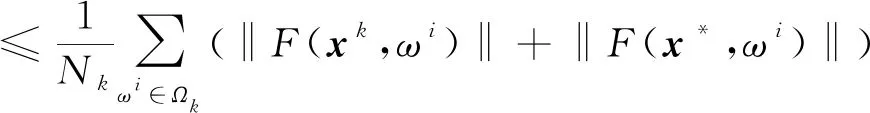
Firstly, we show
(10)
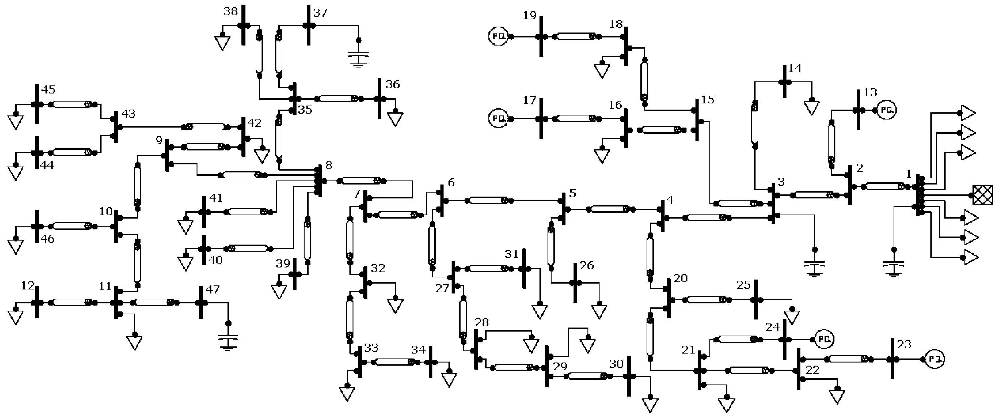
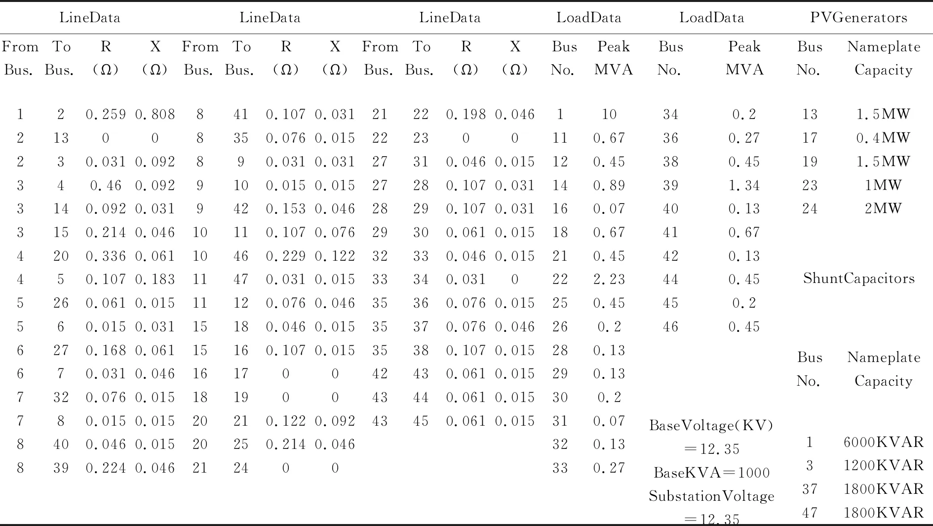
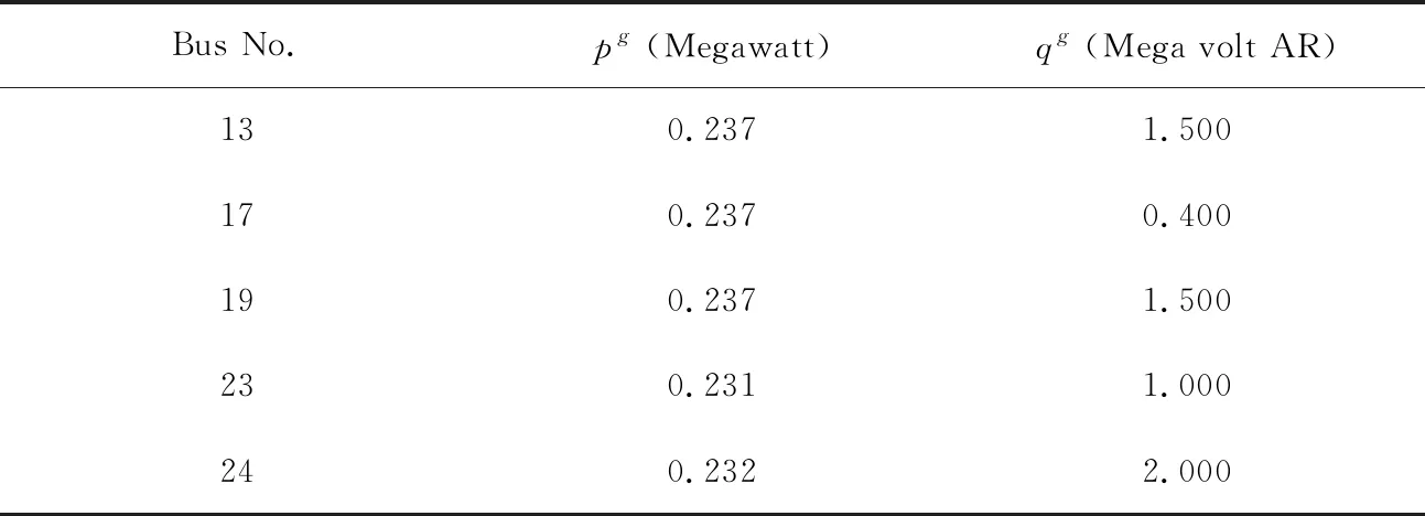
Let E[‖Φ(x*,ω)‖2] ‖Φ(z,ω)-Φ(x,ω)‖≤v(ω)‖z-x‖ holds for allz,x∈n, wherev(ω)>0 is a constant depending onω. Furthermore, we can deduce thatv(ω)≤c1(‖M(ω)‖+‖q(ω)‖) for some constantc1>0. Furthermore, for eachx∈Lh(r), we can deduce that ‖Φ(x,ω)‖≤c2(1+‖x‖)(‖M(ω)‖+‖q(ω)‖) for some constantc2>0. Thus, we have Hence (10) is true. By Theorem 1 and (10), we have Notice that where the equality can be deduced by the mean-value theorem, and the second and third inequalities follow from (7). By (4), we can obtain Taking limitsk→+∞ for both sides of (9), by (4), we can obtain (8), this completes the proof. In this section, a stochastic optimal power flow with radial network structure in power system is considered. It can be reformulated as a stochastic second-order cone programming, which can be deduced by the fact that the convex relaxation of the nonlinear power flow equations has the same form with the rotated second-order cone. Under some conditions, the stochastic second-order cone programming can be solved by its KKT conditions. Since the KKT conditions of the stochastic second-order cone programming optimal power flow problem are a mixed stochastic linear second-order cone complementarity problem, we can employ the solution methods discussed above to solve the stochastic second-order cone programming optimal power flow problem. On each busi∈N, letVibe the complex voltage andsibe the complex net injection, i.e., the generation minus consumption. The power injectionsi=pi+iqiis constrained to be in an pre-specified box constraint setSi. For each line (i,j)∈Ξ, letIijbe the complex current flowing from busesitoj,zij=rij+ixijthe impedance on line (i,j), andSij=Pij+iQijthe complex power flowing from busito busj. As customary, we assume that the complex voltageV0on the substation bus is given. Based on a stochastic OPF model presented in [10], we present next its convex second-order cone branch flow reformulation, which seeks to minimize the generation cost, subject to power flow constraint, power injection constraint, and voltage constraint. This formulation we considered is (11) s.t. si∈Si,i∈N+, Since minf(x) , (12) where the vectorxrepresents all the dispatching random variables related to optimal power flow of the distribution network,f(x) represents the total generation cost, andXis the feasible set of radial distribution network. In order to evaluate the proposed stochastic second-order cone programming optimal power flow problem, a slightly modified version of a real-world 47-bus network in the service territory of Southern California Edison (SCE) with two wind farms connected to bus 9 and bus 30. The SCE network is shown in Figure 1 with parameters given in Table 1. Figure 1 Schematic diagram of SCE 47-bus distribution system Table 1 Network of Figure1: Line impedances,peak spot load KVA,Capacitors and PV generation’s nameplate ratings We suppose that the system regulator is to optimize the total generation cost in an hourly basis in the presence of variable wind power generations by assuming that the forecasted distribution for wind speed is available for the next hour interval. With a fixed parameterτ=1.8, The dispatch results from the day ahead market, which are obtained based on the wind power assuming Gaussianity injected to bus 9 and bus 30 in GAMS platform using NLP solver, are given in Table 2. Table 3 depicts the expected residual and the total generation cost, as the sample size increases. Table 2 OPF results for SCE 47-Bus considering Gaussian wind power uncertainty with 1,000 sampled scenarios Table 3 Expected residual and generation cost considering Gaussian wind power uncertainty We have studied the expected residual minimization formulation for the mixed stochastic linear second-order cone complementarity problem (1). We have discussed the coercive property of the ERM problem and the convergence of the Monte Carlo approximation problem for the ERM problem. Furthermore, we have reported some numerical results by applying the theoretical results to a stochastic optimal power flow with radial network structure in power system. It is worth noting that, in our discussion, we mainly use the generalized Fischer-Burmeister functionφτ. In fact, there are some other second-order cone complementarity functions, which may be used to replace the functionφτ. In the next step, we will try to use the other second-order cone complementarity functions to study the stochastic second-order cone complementarity problem. And since the second-order cone complementarity problems are a generalization of the complementarity problems[12-15], we can use some of the methods to study the problem (1). Acknowledgments: The authors are very grateful to the reviewers for their helpful suggestions and for the inspiration of relevant literatures.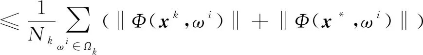

5 Numerical Experiments


6 Conclusions