Classical solutions of the 3D compressible fluid-particle system with a magnetic field

Bingyuan HUANG(黄丙远)

School of Mathematics and Statistics，Hanshan Normal University，Chaozhou 521041，China E-mail: huangby04@126.com Shijin DING (丁时进)+

South China Research Center for Applied Mathematics and Interdisciplinary Studies，School of

Mathematical Sciences，South China Normal University，Guangzhou 510631，China E-mail : dingsj@scnu.edu.cn

Riqing WU (伍日清)

School of Mathematical Sciences，South China Normal University，Guangzhou 510631，China E-mail: 1065334763@qq.com

Recently， the first two authors and Hou [12] studied (1.1) for the 2D Cauchy problem， and derived the local well-posedness of the strong solution. If we remove the magnetic field， model(1.1) turns into the bubbling regime of a compressible fluid-particle model derived by Carrillo-Goudon[5]，called the compressible Navier-Stokes-Smoluchowski system. There are some results on the well-posedness and an asymptotic analysis of the interaction model; Carrillo， Ballew et al.， in papers [1–3， 6]， considered the initial boundary problem in three dimensions， and they obtained the weak solutions， the low-mach number and the low stratification model. Under periodic boundary conditions in two or three dimensions， Huang et al. in [21] considered the incompressible limit of the compressible model. The strong and classical solutions in a 1-D bounded domain were established in [16] and [44]， respectively. For the 3-D Cauchy problem，Chen et al. in [11] and Ding et al. in [13] established the non-vacuum classical solutions， while Huang et al. [15， 20] obtained the local and global classical solutions containing a vacuum.Furthermore， the asymptotic behavior was proved in [15] under the condition of small initial assumptions. For the blowup in a unbounded and bounded domain please refer to the papers[14， 22]. Strong solutions of the 2-D Cauchy problem can be found in the paper [19].

When the factor of particle density in the mixture and the magnetic field are removed，model (1.1) turns into the compressible N-S equations. Work on the well-posedness for the compressible fluid system can be found in [24， 30， 38， 39] for one-dimensional space. Strong or classical solutions to the multi-dimensional problems containing no-vacuum were studied in papers [27， 36， 37， 40]; for the solutions containing a vacuum， please see papers [8–10， 34， 35].Later， Hoff[25， 26] researched the weak solutions，and some studies on the weak solutions were obtained in papers[17， 28，33]. Recently， the 3-D and 2-D Cauchy problems were considered in Xin et al.’s papers [23， 31]; they established the global classical solutions containing a vacuum for when the initial energy is small enough. We also refer to[32，42，43]for results on the global solutions following Huang-Li-Xin’s method in [23].

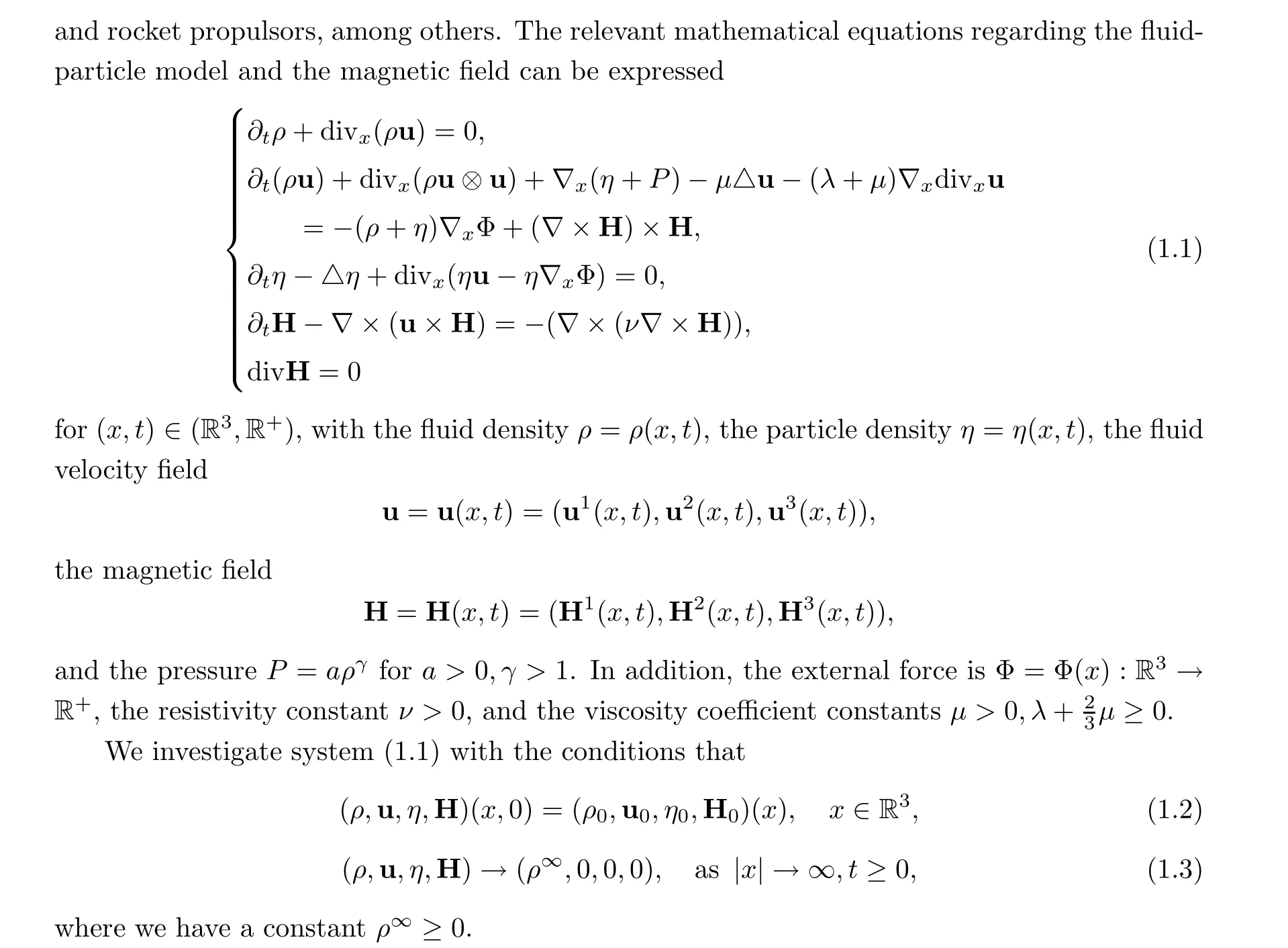
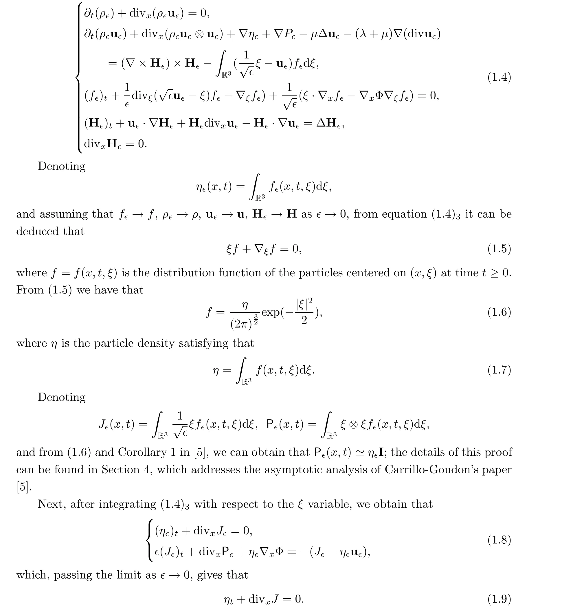
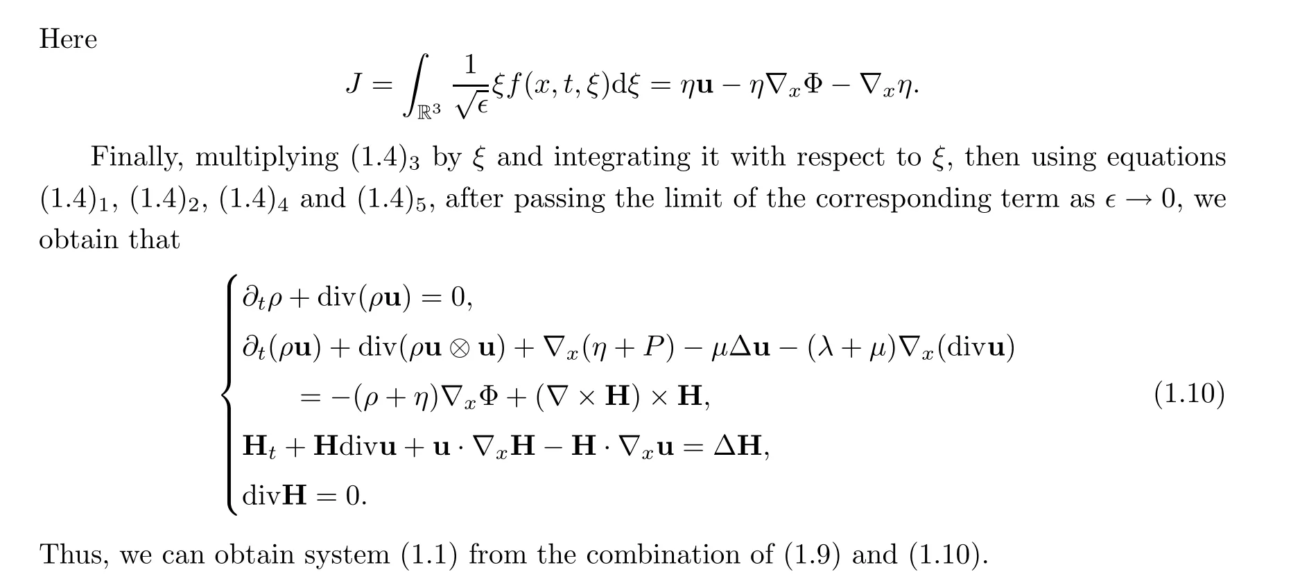
For the convenience of understanding system (1.1)， we will formally derive it from the Vlasov-Fokker-Planck/compressible MHD equations. First， we consider the following asymptotic equations under the idea of asymptotic analysis in [5， 7， 29， 41]:

2 Main Result

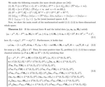
Remark 2.2 If the magnetic field H is ignored，Theorem 2.1 is consistent with Theorems 2.1 and 2.2 in [20]， where a compressible fluid-particle model is considered. Furthermore， if the magnetic field and the particle density are removed from problem (1.1)–(1.3)，Theorem 2.1 is the same as that in [9]. Applying the arguments of Sobolev embedding and the results of Lions-Aubin， we can declare from Theorem 2.1 that (ρ，u，η，H) is a unique classical solution，namely， (ρ，u，η，H)∈C(R3×(0，T0]).

Remark 2.3 The condition e-Φ∈L1(R3) is consistent with that of the initial boundary problem in papers [3， 5， 6]. In this paper， the condition of Φ is used to deal with the term‖η ln η‖L1(R3)from the basic energy estimate， which is similar to that in papers [3， 5， 6]. More precisely， we use e-Φ∈L1(R3) to control the lower bound of ‖η ln η‖L1(R3)， that is，

3 The Results of the Linearized System

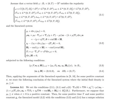
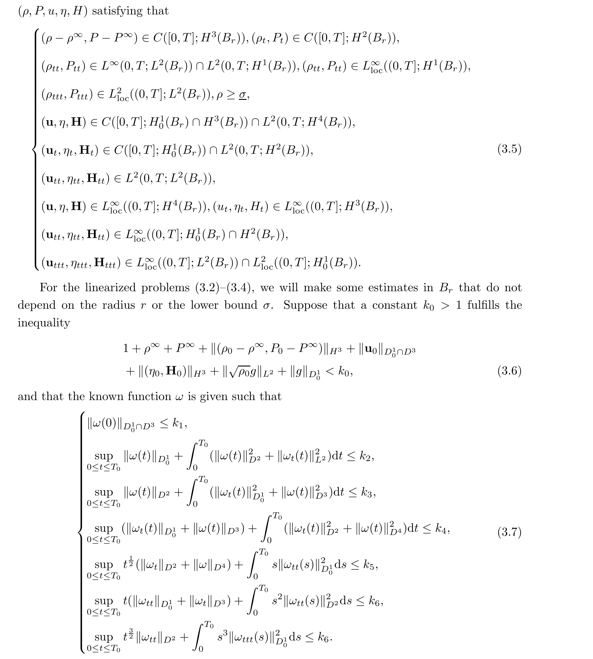
Here 1 ＜k0≤kj-1≤kjfor j =1，2，...，6 and we have T0∈(0，T) with the constants kjand T0to be determined later.

In this section，C is marked as a generic positive constant relying on‖Φ‖H4，ν，µ，γ，λ，T. In addition，suppose that M =M(·):[1，+∞)→[1，+∞)is a fixed increasing continuous function depending only on the constant C.

From Lemmas 3.2 and 5.2 in [9] for the compressible N-S equations， and Lemma 3.3 in

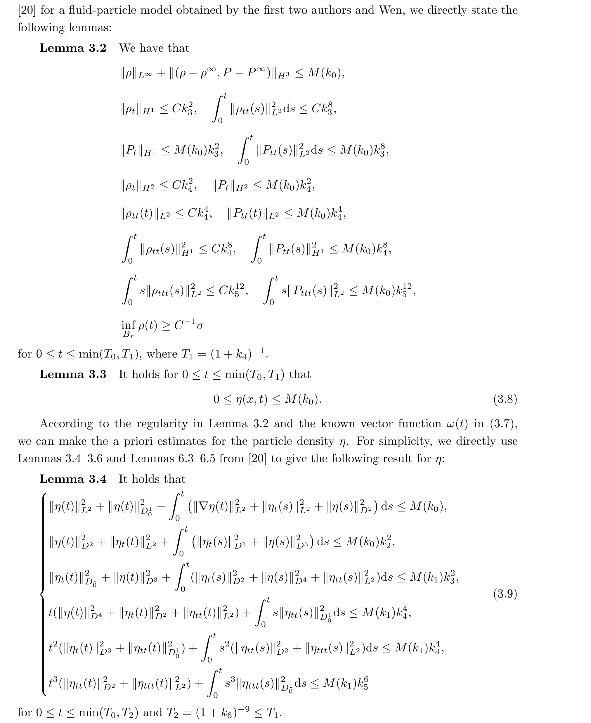
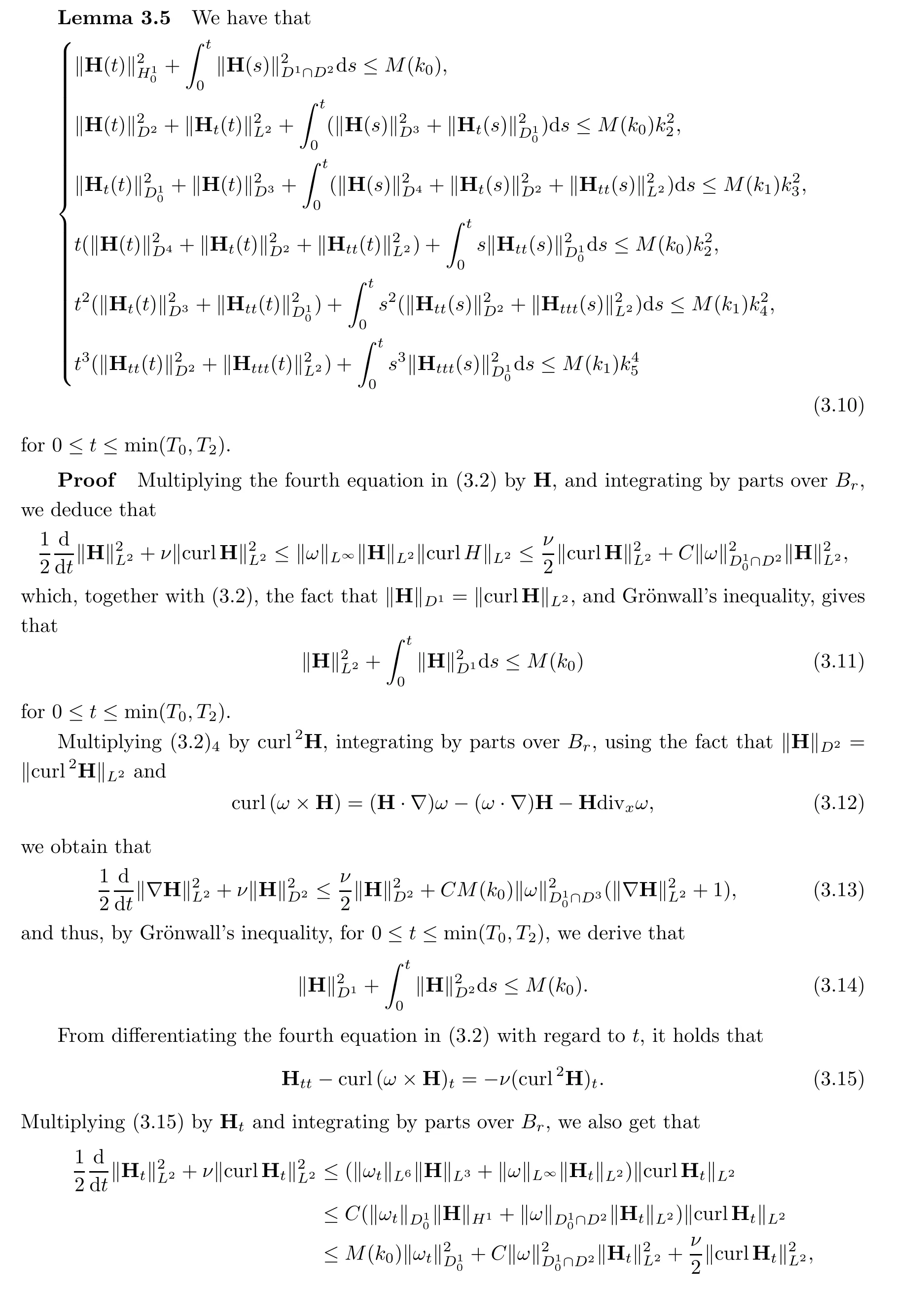
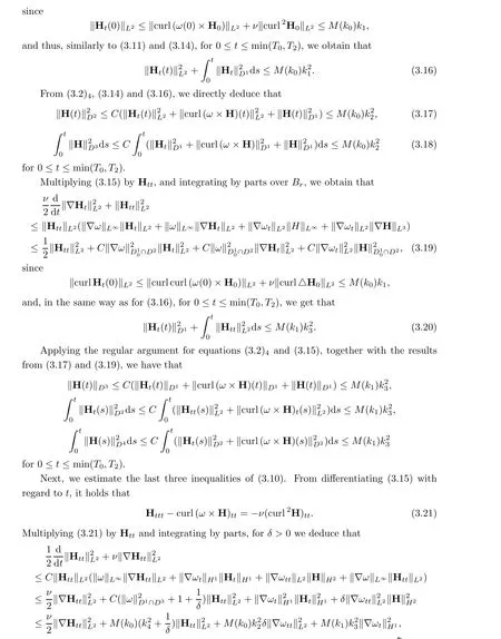
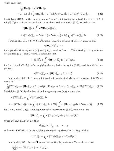
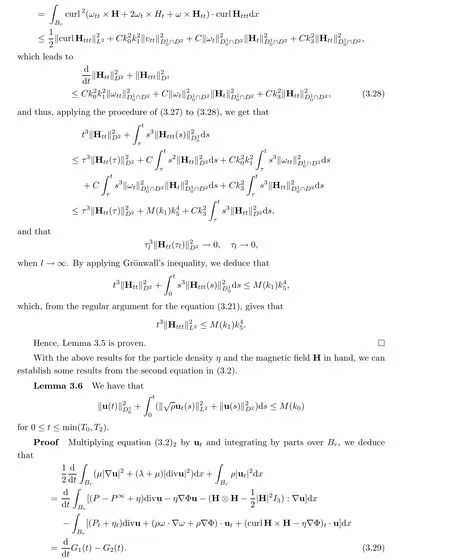
Next， we want to make some estimates for the fluid velocity u and the magnetic field H.In view of equation (3.2)4， we derive some necessary estimates for the magnetic field H.

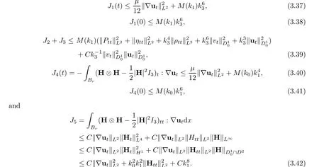
With the estimates from Lemmas 3.2–3.7 in hand， we can derive the estimates of the terms J1(t) and J2using the same procedure as that employed in obtaining the results (65)–(71) in[20]. Hence， it is not necessary to repeat the details of the proofs， and for simplicity， we refer readers to the following results (65)–(71) in [20]:

Thus， applying the argument from Lemma 4.1 in [20] or Lemma 9 in [9]， we establish that the solution of the linearized problem (3.2)， (1.2)–(1.3) has the regularity (2.3).

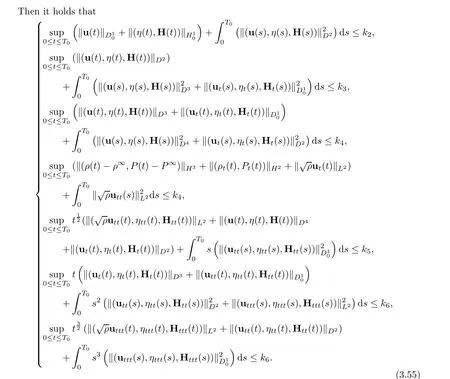
Lemma 3.10 If the initial data (ρ0，u0，η0，H0) satisfies (3.6)， the known vector function ω satisfies regularity (3.1) and estimate (3.7)， where the constants kj(j = 1，2，3，4，5，6) are defined in (3.53) and the time T is replaced by T0. Then the linearized Cauchy problem (3.2)，(1.2)–(1.3) has a unique solution (ρ，P，u，η，H)， together with estimate (3.55) and regularity(2.3).

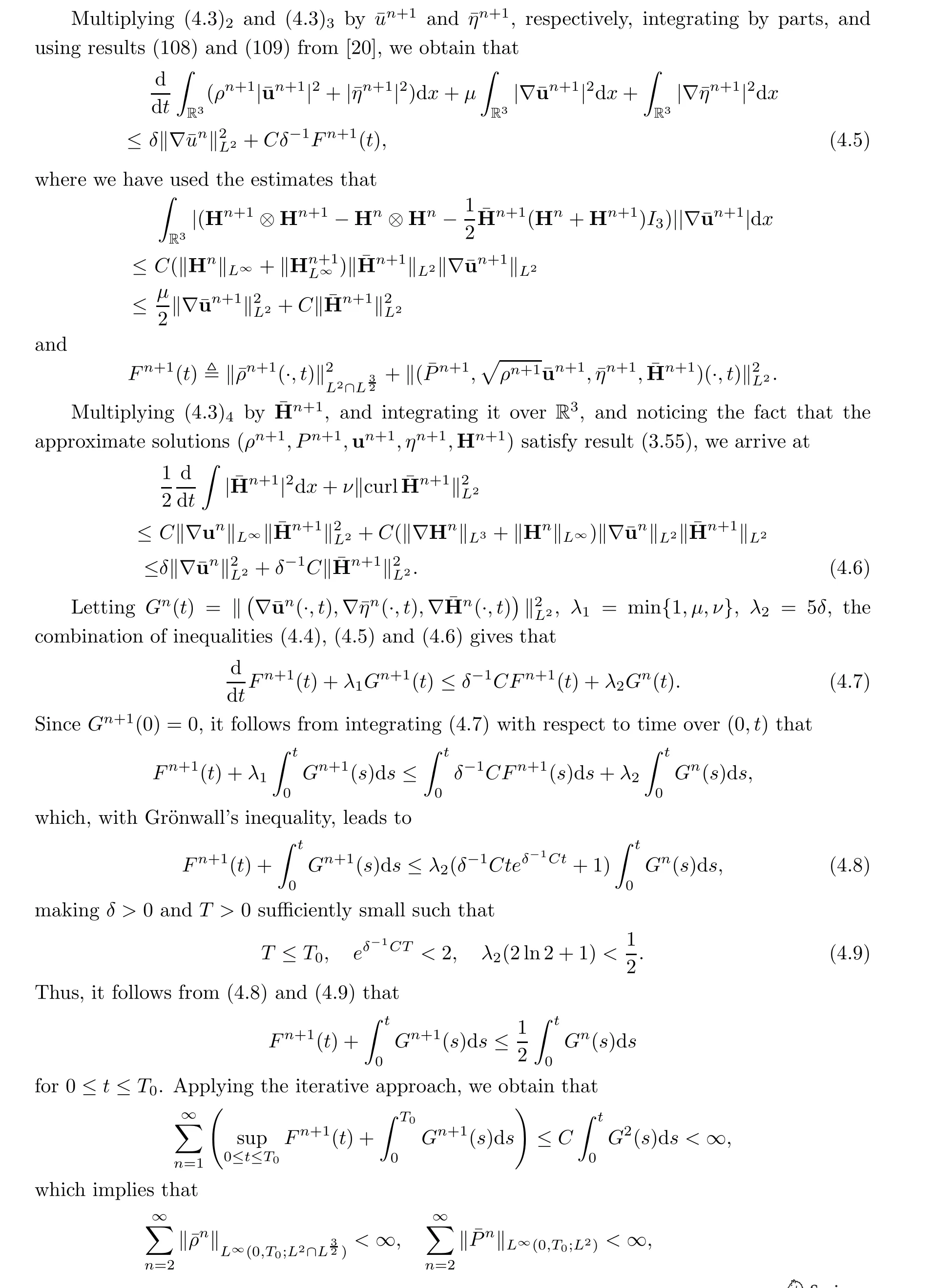
4 Proof of Theorem 2.1

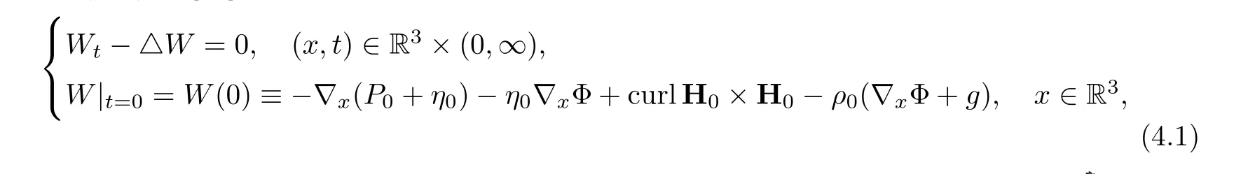
In order to establish the solution to system (1.1)–(1.3)， we will use an inductive argument to consider linearized system (3.2). Following the same process as that used to achieve the result (101) in [20]， we look at the problem

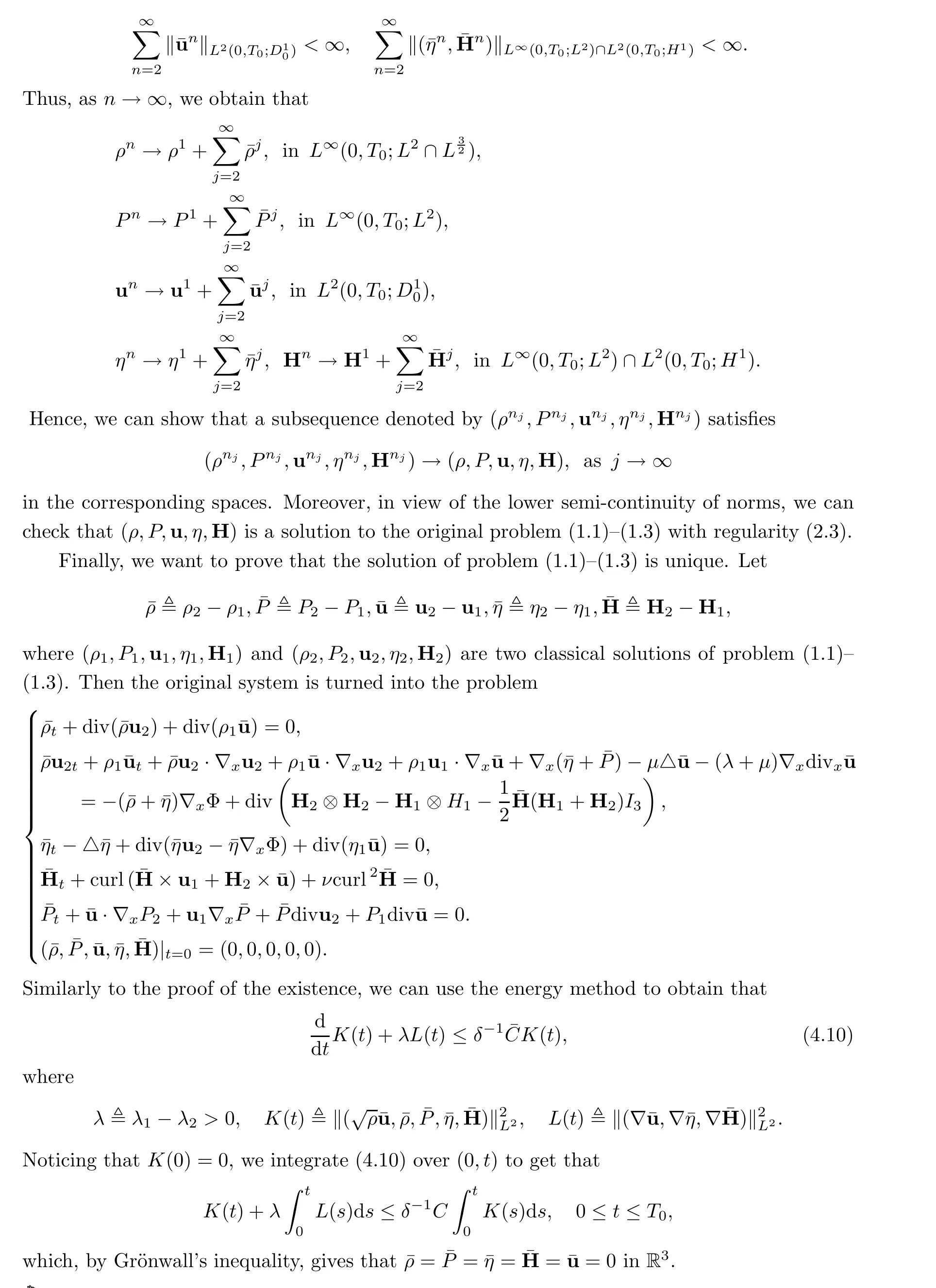
Hence， Theorem 2.1 is proven.

Acknowledgements The first author would like to thank Professor Zheng-an Yao for the useful discussions held at Sun Yat-sen University in 2021.