Global well-posedness of the 2D Boussinesq equations with partial dissipation

Xueting Jin (晋雪婷)t

School of Mathematical Sciences，Capital Normal University，Beijing 100048，China

E-mail: wuetingjin@163.com

Yuelong Xiao (肖跃龙)

School of Mathematics and Computational Science，Xiangtan University，Hunan 411105,China

E-mail : xuyl@atu.edu.cn

Huan Yu(于幻)

School of Applied Science，Beijing Information Science and Technology University,Beijing 100192，China

E-mail : huangu@bistu.edu.cn

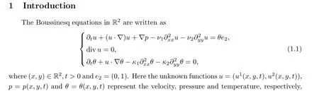
The Boussinesq equations model large scale atmospheric and oceanic flows that are responsible for cold fronts and for the jet stream (see， Majda [24]， Pedlosky [26] and Vallis [28]). In recent years there has been a lot of work on the mathematical theory of the Boussinesq system(1.1). It is well-known that Boussinesq system (1.1)， with all positive viscous and diffusivity coefficients， processes a unique global solution corresponding to sufficiently smooth initial data(see， e.g.， [5， 16， 27]). However， when all viscous coefficients and diffusivity coefficients are zero， system (1.1) becomes inviscid， and the global regularity problem is still completely open.In fact， as pointed out in [25]， the 2D inviscid Boussinesq equations can be identified with the incompressible 3D axi-symmetric Euler equations with swirls.

The Boussinesq equations with partial dissipations， that is， the intermediate cases when some of the parameters are positive， have recently attracted considerable attention. More precisely， Hou–Li [18] and Chae [10] proved the global well-posedness of system (1.1) with full viscosities but without any diffusivity. In addition， Chae [10] also proved the global wellposedness of system (1.1) with full diffusivity but without viscosities. The initial data in[10， 18] is required to satisfy some appropriately higher regularity. Later， some generalizations of [10， 18] were obtained by Hmidi–Keraani[17] and Danchin–Paicu[13]. In particular，in [13]，the initial data is only assumed to be in L2(R2). The corresponding initial-boundary value problem was studied in [19] and [20]. Very recently， Danchin–Paicu [14] and Larios–Lunasin–Titi [21] examined system (1.1)with only horizon viscosity (that is， ν1＞0， ν2=κ1=κ2=0)，and obtained the global well-posedness with the initial data satisfying appropriately higher regularity. However， this is unclear for the case with merely a vertical viscosity， namely， where ν2＞0 and ν1= κ1= κ2= 0. Futhermore， for when ν2＞0 and κ2＞0 (ν1= κ1= 0 meanwhile)， Cao–Wu [9] proved that system (1.1) has a unique global classical solution if the initial data belongs to H2(R2). The initial conditions were relaxed by Li–Titi[22]for when the initial data belongs to the space X ={f ∈L2(R2)|∂xf ∈L2(R2)}.

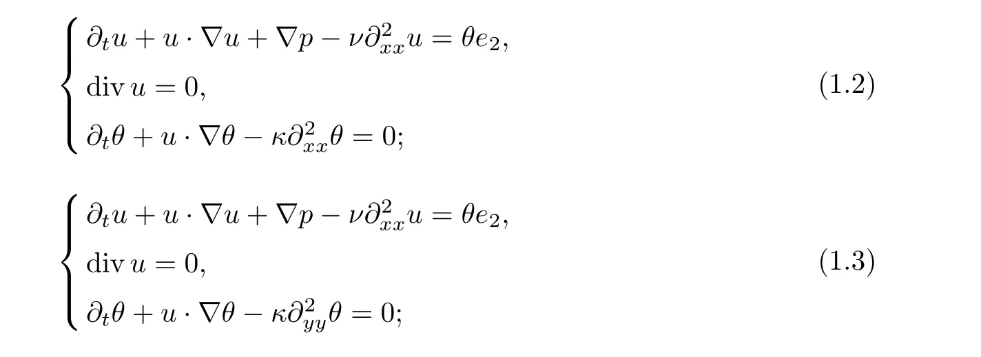
Inspired by [22]， where Li-Titi dealt with the case ν2＞0， κ2＞0 (ν1=κ1=0)， we intend to explore three other kinds of particular dissipation cases. More precisely，we will consider the global well-posedness of the other cases under lower regularity of the initial data，that is，where we have the following: ν1＞0， κ1＞0 (ν2= κ2= 0); ν1＞0， κ2＞0 (ν2= κ1= 0); ν2＞0，κ1＞0(ν1=κ2=0). Indeed， for when the initial data satisfies appropriately higher regularity，the global well-posedness of the three cases has been proved in[11]. Our goal here is to weaken the hypothesis in[11]with respect to the initial data as much as possible. To simplify，the three systems under consideration can be written as

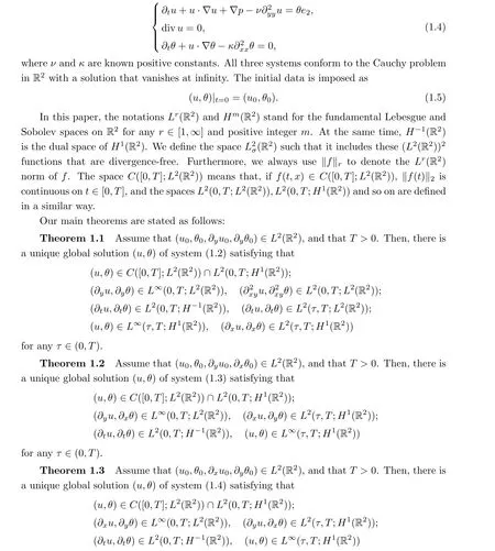
for any τ ∈(0，T).

Remark 1.4 (i) Theorem 1.1，Theorem 1.2 and Theorem 1.3 are generalizations of those in [11]， where the initial data is required to be in H2(R2).

(ii) As will be seen later， the regularity regarding the derivative of one of the directions(x，y) to the initial data is required to ensure uniqueness. Since the systems we consider lack some direction dissipations， our hypothesis regarding the initial data is natural.

(iii) Our results are applicable for the periodic boundary conditions as well.

We get a local well-posedness result by adding the lacking dissipation in a corresponding system with lower regularity of initial data. Moreover， the anisotropic inequality is used suffi-ciently to overcome the difficulty caused by partial dissipation. In addition， we prove a global H1estimate in a standard way. In the end， we get the global well-posedness result with lower initial data by the extension of the solution. At the same time， our initial data ensures the uniqueness result.

For the readers’ convenience， anisotropic inequality is stated as follows:

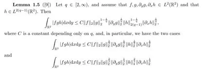
for an absolute positive constant C.

In what follows， we briefly assume that ν =κ=1. Throughout this paper， C stands for a general positive constant.

The rest of this paper is arranged as follows: in Section 2， we establish the global wellposedness of system(1.2)with lower regularity of initial data. In Section 3，we prove the global well-posedness of system (1.3)， and that of system (1.4) with lower regularity of initial data.

2 Proof of Theorem 1.1

This section is devoted to proving Theorem 1.1，and it is divided into two subsections. The first subsection proves the global well-posedness result with H1initial data; this will be used to prove Theorem 1.1 in the second subsection.

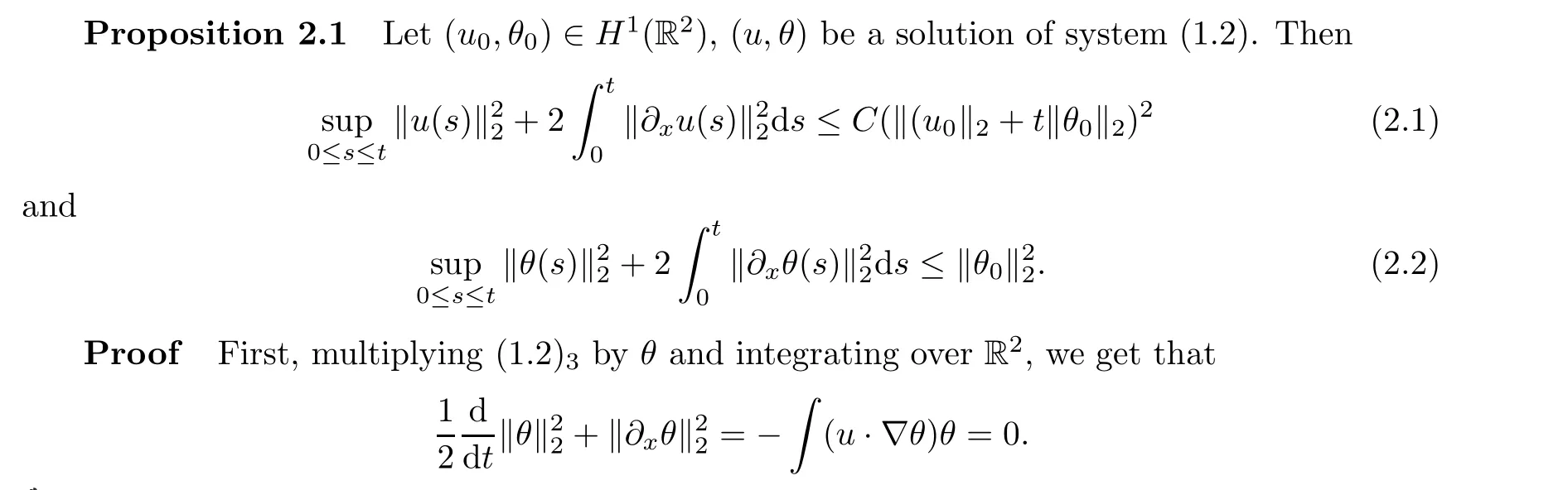
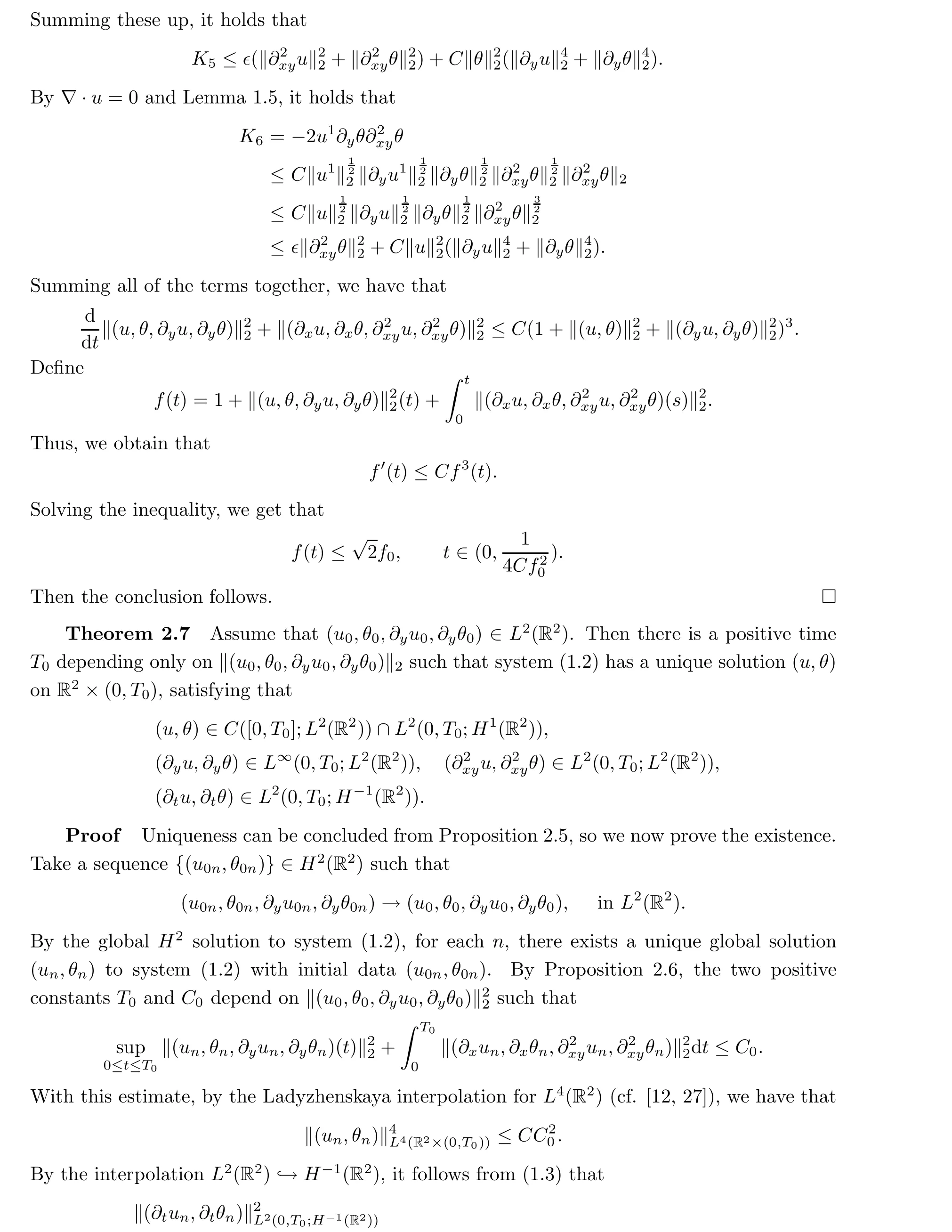
For the proof of the global well-posedness with H1initial data， for simplicity， we only give some of the bounds. We begin with the basic energy estimates.

2.1 Global well-posedness: H1 initial data

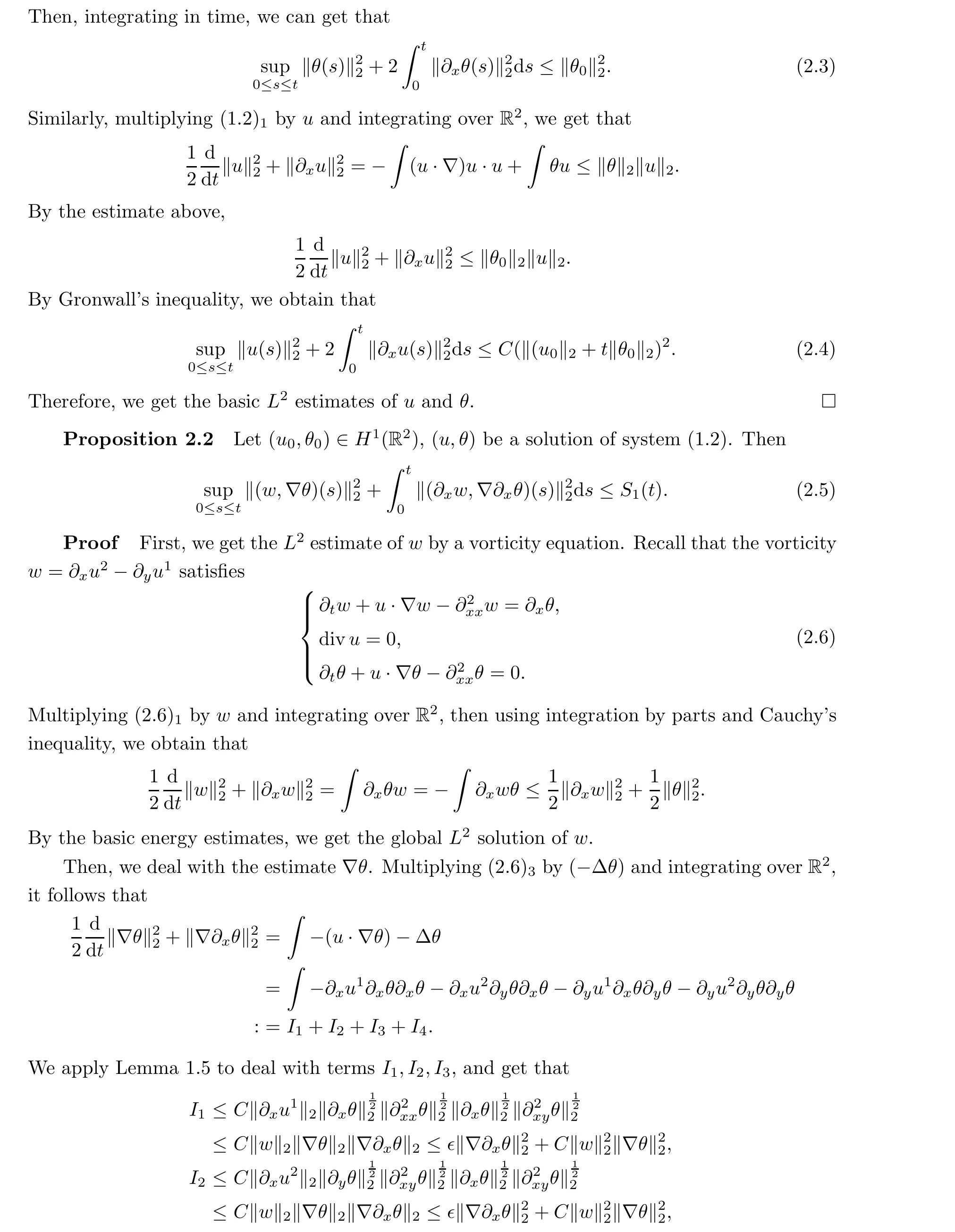
and

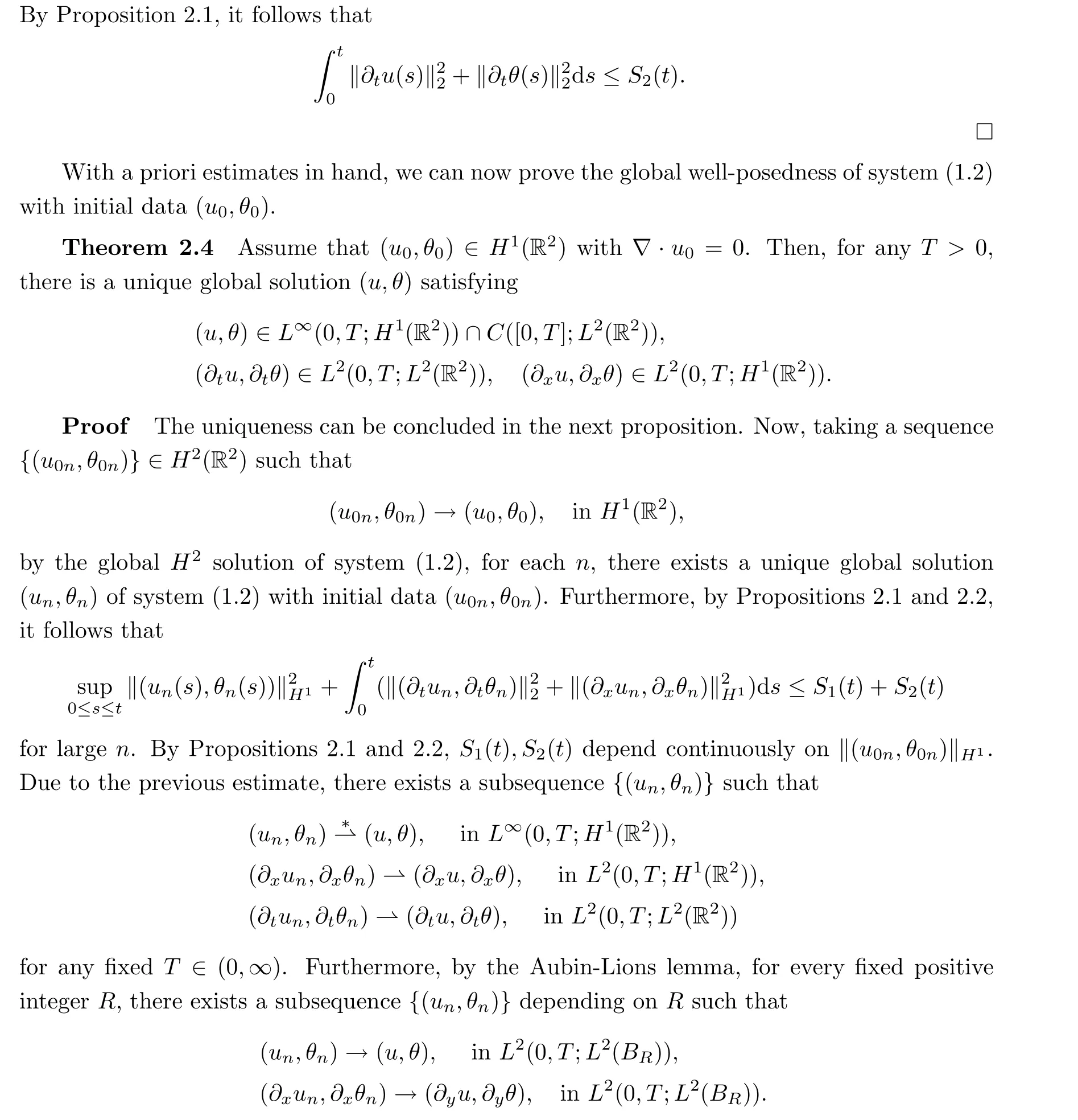
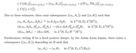
By these convergences，we can use the diagonal argument in n and R，and from the subsequence denoted by {(un，θn)}， there are (un，θn) →(u，θ) in L2(0，T;(L2(Bρ)) and (∂xun，∂xθn) →(∂xu，∂xθ) in L2(0，T;(L2(Bρ)) for arbitrary ρ ∈(0，+∞)， thus (u，θ) is a global solution that satisfies the equation in the sense of distribution to system (1.2) with initial data (u0，θ0). In addition， the regularities stated in the theorem follow from the weakly lower semi-continuity of the relevant norms. □

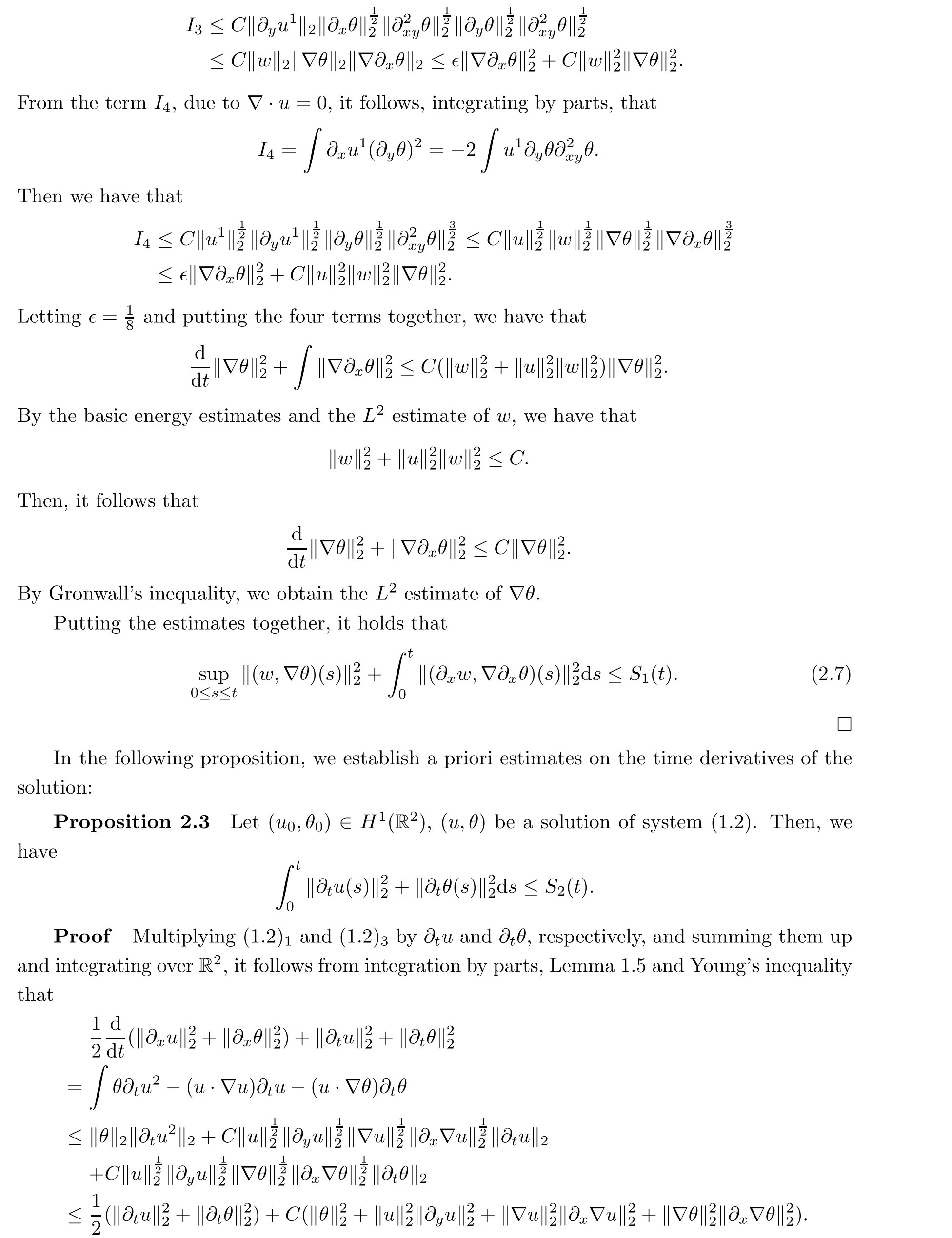
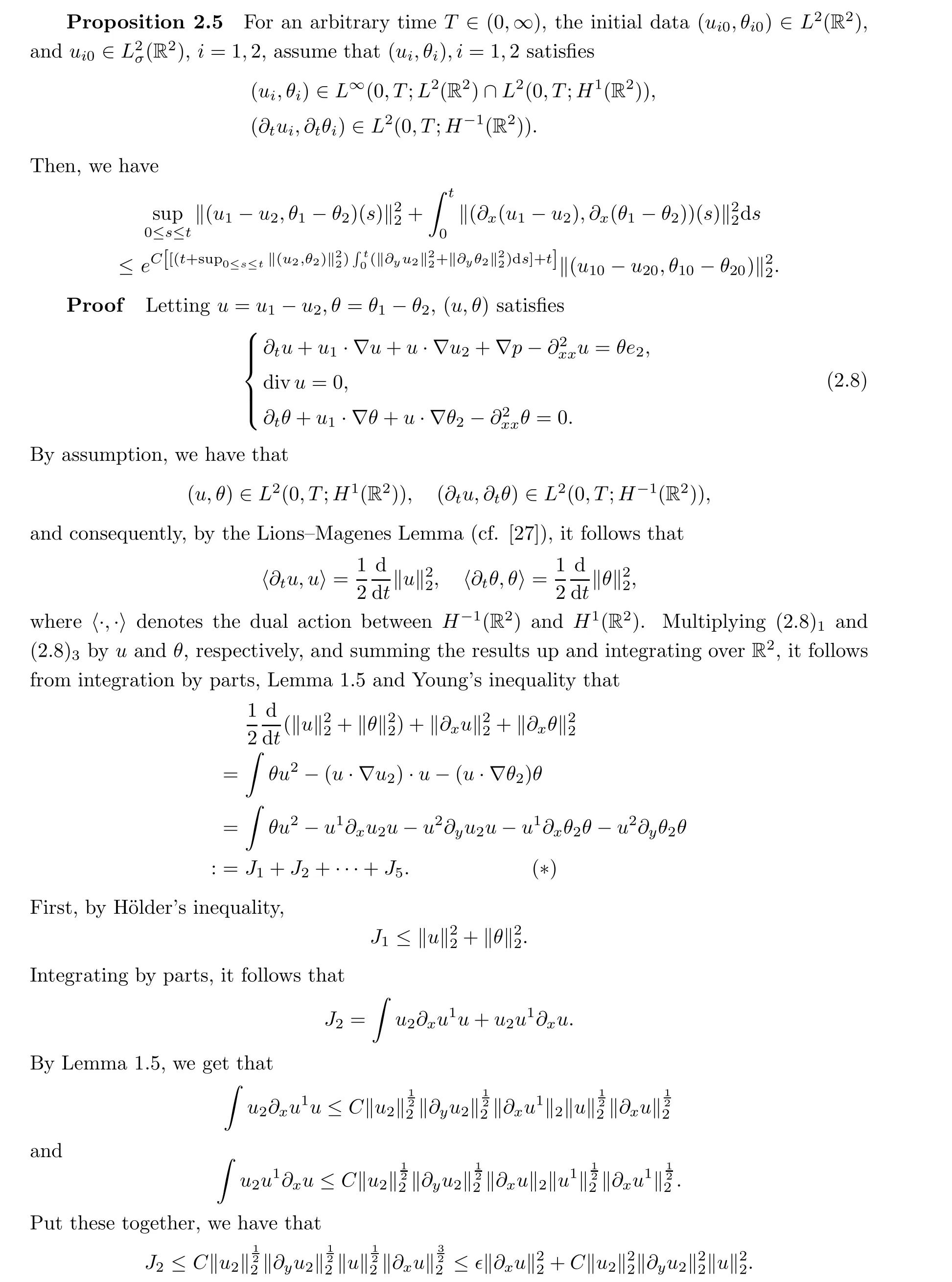
In the next Proposition， we weaken the hypothesis on the regularity of the solution， in particular on their time derivatives， in order to apply the same hypothesis for obtaining the uniqueness of the solutions obtained in preceding H1estimates， as well as those in a later Proposition.

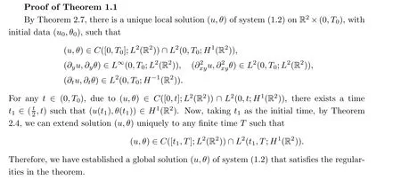
2.2 Proof of Theorem 1.1

By these convergence results， we can use same method as that used to prove Theorem 2.4 to get the global solution. □

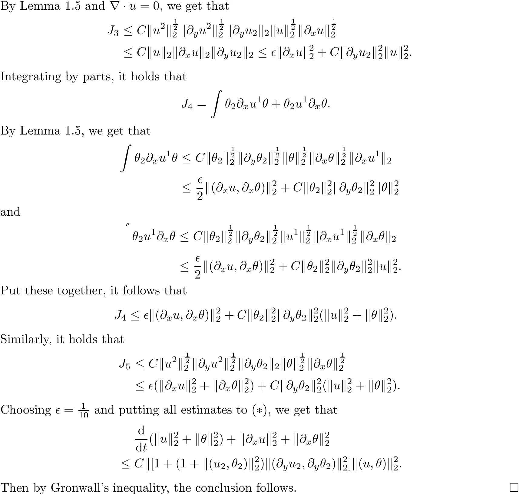
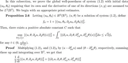
We are now able to prove the global well-posedness of system(1.2)with lower regular initial data.

3 Proofs of Theorem 1.2 and Theorem 1.3

This section is devoted to proving Theorems 1.2 and 1.3. It isdivided into three subsections.In the first subsection，we state the basic energy estimates and the known global H2estimates.In the second subsection， we prove Theorem 1.2. In the last subsection，we prove Theorem 1.3.

3.1 Global well-posedness

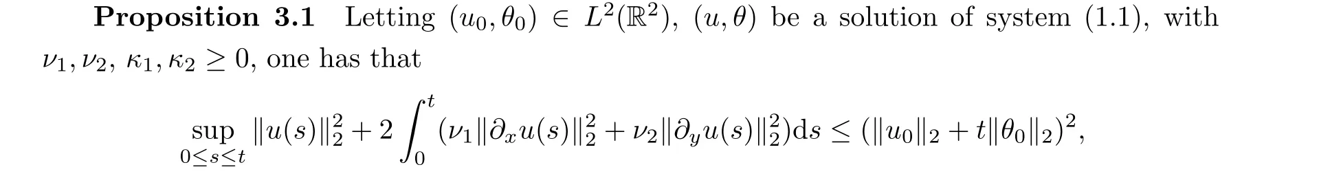
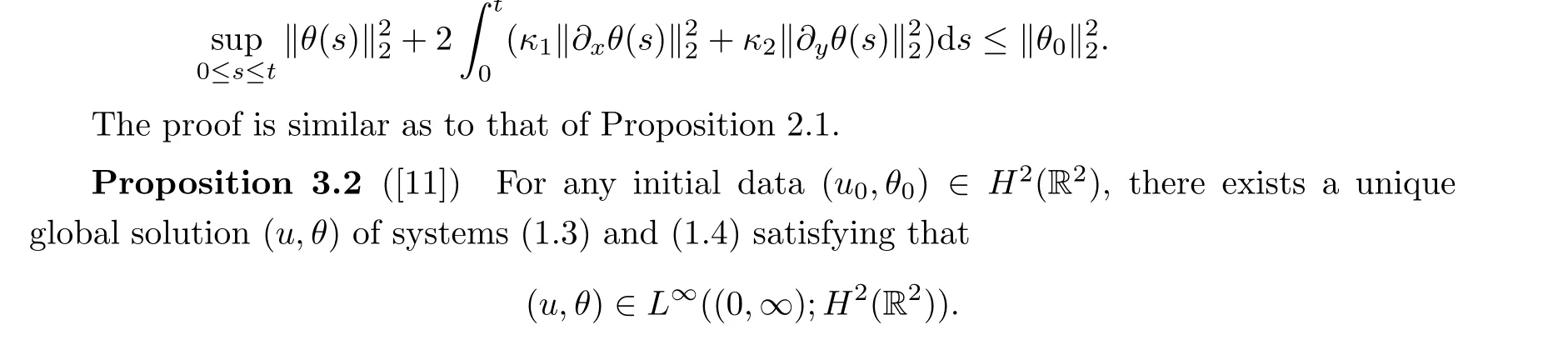
First，we state the basic energy estimate of system(1.1)，with initial data(u0，θ0)∈L2(R2).

3.2 Proof of Theorem 1.2

This subsection is devoted to proving Theorem 1.2; we begin with the H1estimate.

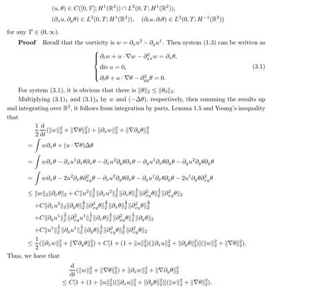
Theorem 3.3 Let(u，θ)be a solution to system(1.3)，with initial data(u0，θ0)∈H1(R2).Then， we have that

for an absolute constant C， which indicates the conclusion. □

The uniqueness estimate is similar to that of Proposition 2.5，so we omit it here. In addition，we can use the same method as was used for proving Theorem 1.1 to get the global solution.

3.3 Proof of Theorem 1.3

We first show the corresponding H1estimate of system (1.4).

Theorem 3.5 Let(u，θ)be a solution of system(1.4)，with initial data(u0，θ0)∈H1(R2).Then， we have

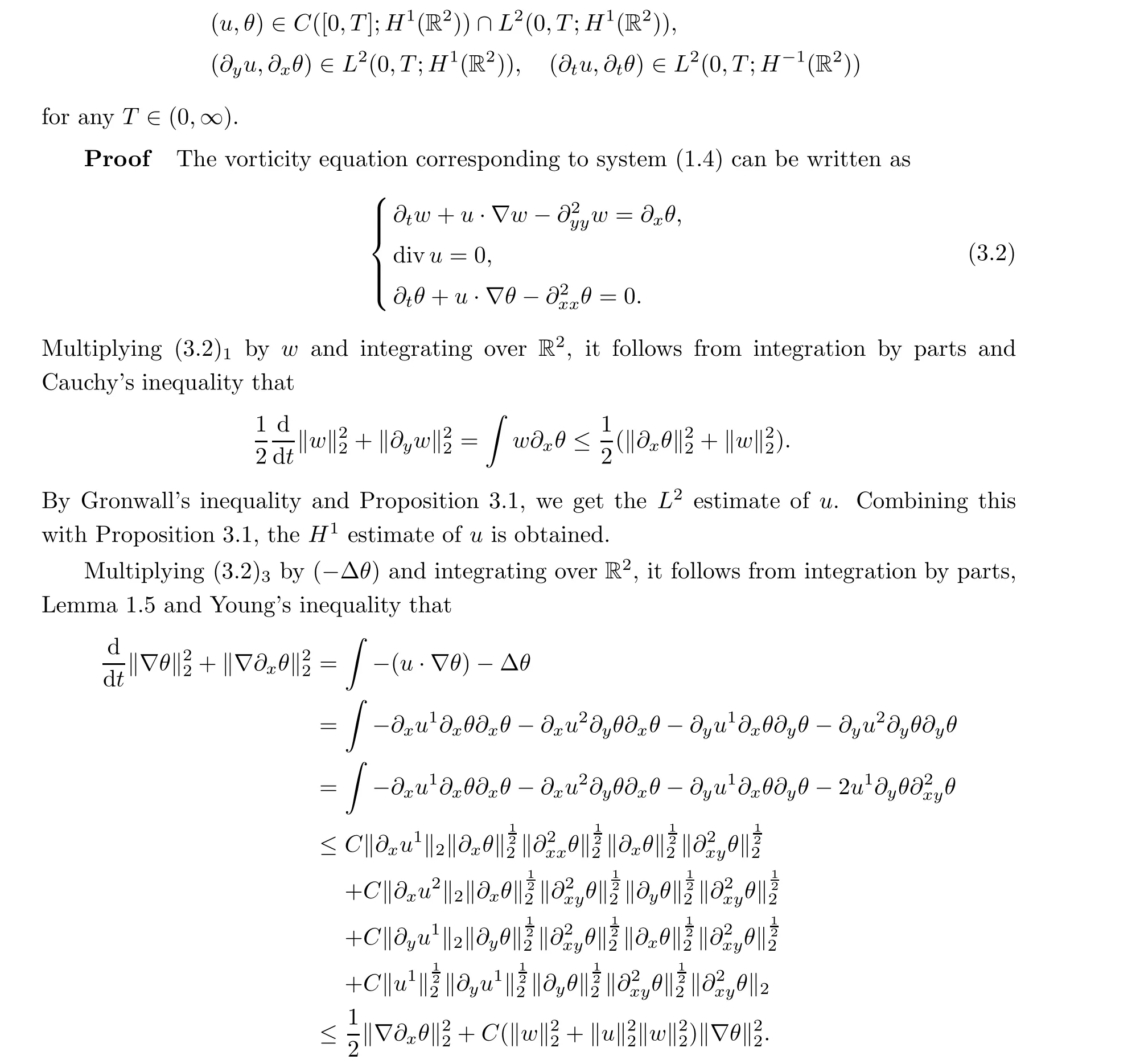
By Proposition 3.1 and the estimates above， we have that ‖w‖22+‖u‖22‖w‖22≤C. Integrating in time， together with Proposition 3.1， yields the conclusion. □

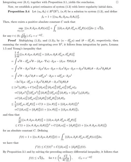
Now， we show the result with lower regularity initial data.

Proposition 3.6 Letting (u，θ) be a solution of system (1.4)， with initial data (u0，θ0)∈H2(R2) and divu0=0， we denote that

for an absolute constant C， which indicates the conclusion. □

In the end， with the above two crucial priori estimates， we can use the same procedure as was used for proving Theorem 1.1 to get the global solution. We omit the details of this here.