Genetic Nelder-Mead neural network algorithm for fault parameter inversion using GPS data

Leyang Wang , Ranran Xu , Fengbin Yu

a Faculty of Geomatics, East China University of Technology, Nanchang 330013, China

b Faculty of Industrial Safety and Occupational Health, Jiangsu College of Safety Technology, Xuzhou 221000, China

c Key Laboratory of Mine Environmental Monitoring and Improving Around Poyang Lake, Ministry of Natural Resources, Nanchang 330013, China

d BGI Engineering Consultants Ltd., Beijing 100038, China

Keywords:Fault parameter inversion Genetic algorithm Nelder-Mead simplex algorithm Neural network algorithm

ABSTRACT The traditional genetic algorithm (GA) has unstable inversion results and is easy to fall into the local optimum when inverting fault parameters. Therefore, this article considers the combination of GA with other non-linear algorithms in order to improve the inversion precision of GA. This paper proposes a genetic Nelder-Mead neural network algorithm (GNMNNA). This algorithm uses a neural network algorithm (NNA) to optimize the global search ability of GA. At the same time, the simplex algorithm is used to optimize the local search capability of the GA. Through numerical examples, the stability of the inversion algorithm under different strategies is explored. The experimental results show that the proposed GNMNNA has stronger inversion stability and higher precision compared with the existing algorithms. The effectiveness of GNMNNA is verified by the Bodrum-Kos earthquake and Monte Cristo Range earthquake. The experimental results show that GNMNNA is superior to GA and NNA in both inversion precision and computational stability.Therefore,GNMNNA has greater application potential in complex earthquake environment.

1. Introduction

The occurrence of earthquakes often brings huge disasters to human production and life. However, since earthquakes occur underground,they lack certain regularity in terms of time and space.Therefore, we lack an in-depth understanding of earthquakes and cannot achieve effective earthquake prediction and protection.But using geodetic data to invert fault parameters helps us study the mechanism of earthquakes. Thereby we can have a deeper understanding of earthquakes. The existing researches are mostly based on the inversion of fault parameters based on dislocation theory.Steketee[1]was the first person to apply the dislocation theory to seismic fault motion.Okada[2,3],on the basis of summarizing the predecessors,linked the fault parameters with the observations of surface deformation and proposed a more general fault dislocation analytical model.

There are two types of methods for solving fault parameters.One is the linearization method,such as the quasi-Newton method[4,5], the steepest descent method [6], and the conjugate gradient method [7], least square method [8], etc. The other is a nonlinear method, such as simplex algorithm [9-11], particle swarm algorithm [12,13], artificial neural network algorithm [14,15], GA[16-19],simulated annealing[20-23],simulated atomic transition algorithm [24,25], homotopy method [26-28], and so on. Because the linearization method relies heavily on the initial solution, and the linearization of the model involves complex derivative calculations.Therefore,nonlinear methods are often used to invert fault parameters. Different nonlinear methods have their advantages and disadvantages.Although the simplex algorithm converges fast,it relies on the initial solution to a greater degree[29].Although the particle swarm algorithm has a fast calculation speed, the calculation result is unstable [29]. The artificial neural network algorithm requires a large number of training samples in the initial stage of calculation, which is not easy to achieve in earthquakes.Genetic algorithm is a kind of bionic optimization algorithm,which obtains excellent offspring by simulating the process of gene selection, crossover, and mutation. Holland [16] proposed the algorithm for the first time, and Stoffa and Sen [17] used it for seismic wave inversion, which is often used to solve seismic source parameters[30,31].And the algorithm is not critical to the use of data;inversion can use either GPS data or InSAR data. However, the current source parameter inversion algorithms mostly rely on InSAR data for inversion calculation [29], while geodetic data includes GPS data and seismic wave data in addition to InSAR data.The efficient use of these two data in source parameter inversion remains studied. In order to fully explore the application value of GPS data for seismic source parameter inversion,we consider using GA for inversion calculation. But the genetic algorithm operation process has strong heredity,so the effective gene,once lost,is very difficult to recover, prone to the premature phenomenon. Therefore,we consider improving the genetic algorithm [32-34].

Sadollah et al.[35]proposed a neural network algorithm,which simulates the process of information transmission by neurons in the human brain, and can adaptively summarize the rules and complete some operations.However,at present,the application of this algorithm in fault parameter inversion is less,so the inversion of fault parameters by this algorithm needs to be explored. The simplex algorithm has a fast convergence speed but strong dependence on the initial value. Therefore, this paper considers using a neural network algorithm to make up for genetic easy to fall into local optimum defects. At the same time, the simplex algorithm is used to optimize the ability of the genetic algorithm to further find the optimal solution.In order to improve the inversion precision of the genetic algorithm and fully tap the application value of GPS data in seismic source parameter inversion,this paper proposes a genetic Nelder-Mead neural network algorithm(GNMNNA). Numerical examples and two real earthquakes verify that the proposed algorithm has a wide range of applications in fault parameter inversion,fast convergence,and stable and reliable calculation results.

The second section of this paper introduces the nonlinear search algorithm for fault parameter inversion;the third section proposes an improved GA;the fourth section verifies the validity of GNMNNA through numerical examples and real earthquakes;the fifth section is giving a summary based on experimental results.

2. Nonlinear search algorithm for fault parameter inversion

2.1. Fault parameter inversion

Okada elastic dislocation theory[2,3]uses mathematical models to link geodetic data with fault parameters and provides an important means for inverting fault parameters from geodetic data.Fault parameters include geometric parameters(coordinates of the center of the fault plane,fault length,width,strike,dip,depth of the fault center) and slip parameters (rake and slip). The relationship between fault parameters and surface deformation is as follows:

where d is the observed deformation of the surface, m is the fault parameter,G(·)is the nonlinear mapping of the fault parameter to the surface deformation, and ε is the observation error of the deformation.

In the process of fault parameter inversion, the root mean square(RMS)between the observed and predicted values of surface deformation is usually used to construct the objective function.The form is as follows:

where n represents the number of surface observations, q represents the weight of each observation, d represents the observed value of surface deformation,and c represents the predicted value of surface deformation.

2.2. Genetic algorithm (GA)

The genetic Algorithm [16,17,30,31] was first proposed by Professor Holland of Michigan University in the United States.The algorithm is a heuristic search algorithm which selects the best individual through the survival of the fittest mechanism. In the inversion of fault parameters based on GA, the interval of fault parameters needs to be determined based on prior information.Then encode the parameter interval,that is,transform one problem into another in some way.Randomly generate the initial population in the encoded parameter interval,and then calculate the objective function value of each body in the population, namely RMS, and arrange the individuals in order of good or bad. In the wellarranged population, select the better individuals to cross in pairs, that is, to exchange part of the chromosomes between the two individuals with a certain probability. Finally, individual mutations are made according to a certain probability to prevent falling into extreme values. It gradually converges to the optimal individual through repeated selection, crossover, and mutation operations. The specific implementation process is as follows; the algorithm flowchart is shown in Fig.1:

1. Given the population size N,the maximum number of iterations iter, the crossover rate P, the mutation rate P, the parameter interval [lb ub];

2. Encode and generate the initial population M;

3. Calculate the fitness function of the population to distinguish the good differences among individuals;

4. According to the calculated individual fitness function, arrange them in order of good or bad, and select the individuals with good fitness as the parents to reproduce the offspring;

5. Select two individuals in the parents,and exchange part of their chromosomes with a certain probability Pto generate a new individual;

6. Make individual mutations with a certain probability Pto generate a new population;

7. Calculate the objective function value RMS of the new population,and use the individual with the smallest RMS as the optimal value;

8. Judge whether the iteration condition t ≥iteris satisfied; if yes, jump out of the iteration and output the parameter solution; if not,return to 3;

9. Output parameter solution.

2.3. Neural network algorithm (NNA)

Sadollah et al. [35] proposed an optimization method inspired by the biological nervous system and artificial neural network-NNA. The algorithm connects the parameter solutions through connection weights, continuously updates the parameter solutions,and selects the optimal solution as the target solution to reduce the difference between the target data and the predicted data,and is used to solve the minimum problem.The main process of the algorithm is as follows:

Fig.1. The flow chart of the GA.

First, generate the initial population M:

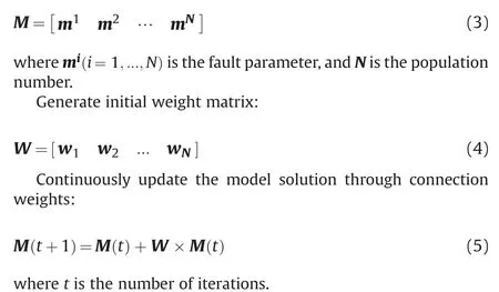
Calculate the objective function value RMS of each parameter solution,take the parameter solution corresponding to the smallest objective function value as the target solution m, and the weight corresponding to the target solution as the target weight w, and continuously update the connection weight through the target weight:

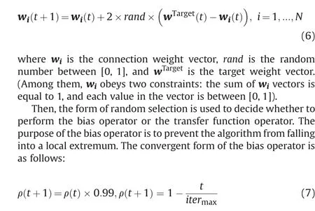
where ρ is the modification factor, which determines the percentage of model solutions that should be modified, and iteris the maximum number of iterations.

Finally, perform the transfer function operator to update and generate the parameter solution closer to the target solution. The updated form is as follows:

By continuously updating the connection weights and parameter solutions until the iterative conditions are met,it breaks out of the loop.The specific calculation steps are as follows,the algorithm flowchart is shown in Fig. 2:

1. Given the number of populations N, the maximum number of iterations iter, the parameter interval [lb ub];

2. According to the parameter interval, the initial parameter solution matrix M is uniformly generated randomly,and the initial weight matrix W is randomly generated;

3. Calculate the objective function value RMS of each parameter solution according to the formula, and use the parameter solution with the smallest objective function value as the target solution m,and its corresponding parameter weight as the target weight w;

4. Generate a new model solution according to equations (5) and(6), and update the connection weights;

5. Generate a random number rand, if rand ≤ρ, perform bias calculation, otherwise perform transfer function calculation according to equation (8);

6. Update according to equation (7), calculate the objective function value RMS of all new model solutions, and judge whether the current minimum objective function value is less than the objective function value corresponding to the target solution;if so, update the target solution mand its corresponding target weight w; otherwise, do not update;

7. Judge whether the iterative condition t ≥iteris met; if it is met,it will exit the iteration and output the target solution;if it is not met, return to 4;

8. Output target solution m

2.4. Nelder-Mead algorithm (NMA)

The core idea of NMA[10]is to randomly generate v+1 points to construct a simplex and v is the dimension of unknown parameters.The simplex points are arranged according to the size of the objective function value,and the last point is the worst vertex.Use points other than the worst vertex to form the centroid, and extend from the worst vertex to the centroid to form the search direction.Along the search direction,four operations of reflection,expansion, outer compression, and inner compression are performed to find the improved vertices. And replace the worst vertex with the improved vertex, repeat it, and get the optimal solution.If a better solution is given as the initial solution of NMAand the inversion calculation is performed, it can often find the optimal solution quickly.

3. Improved genetic algorithm

GA [36] is a heuristic search method with high convergence speed and convergence ability and is often used to solve earthquake fault parameters [30,31]. However, due to the strong heritability during the GA operation,it is difficult to recover the effective genes once they are lost,which leads to premature convergence of GA and falls into the local optimum. In order to effectively improve the situation that GA is easy to fall into local optimum, this paper considers combining GA with other nonlinear search algorithms.NNA[35]is a global search algorithm.NNA simulates the process of information transmission by neurons in the human brain and can self-adaptively summarize rules and complete certain operations.However, at present, NNA is rarely used in fault parameter inversion, so the use of NNA to invert fault parameters needs to be explored. NMA [10] is a local optimization algorithm with a faster convergence speed and stronger convergence ability. However,NMA is strongly dependent on the initial value. The higher the initial value accuracy, the stronger the global search ability.Conversely, the lower the global search capability. Taking into account the adaptive global convergence capability of NNA and the strong local search capability of NMA, this paper designs three combined schemes. The first is the genetic neural network algorithm (GNNA): Combine the adaptive NNA with GA in order to retain the genetic characteristics of GA and at the same time have the ability to adaptively obtain the global optimum. The second is the genetic Nelder-Mead algorithm (GNMA): Combine NMA with GA,and use the local search capability of NMA to further search for the global optimal solution on the basis of GA. The third is GNMNNA:Combine the three algorithms of GA,NNA, and NMA to achieve the effect of complementing each other. Since the combining steps of the three algorithms are roughly similar, this article only gives the specific implementation steps of GNMNNA.GNNA and GNMA are only shown in the flowchart (Fig. 3).

3.1. Genetic Nelder-Mead neural network algorithm (GNMNNA)

Here, the three methods are combined into one algorithm-GNMNNA. First, the selection crossover operation in GA is combined with NNA so that the algorithm has both genetic characteristics and global adaptive capabilities. And because of the special structure of NNA,a target solution will be generated in each iterative calculation.The target solution is the optimal solution for the current iteration. Taking into account the local convergence ability of NMA, the target solution is used as the initial solution of NMA to further search for a better solution. The specific implementation steps of GNMNNA are as follows:

1. Given the number of populations N,the maximum number of iterations iter, the parameter interval [lb ub];

2. According to the parameter interval, the initial parameter solution matrix M is uniformly and randomly generated.Generate the initial weight matrix W;

3. Calculate the objective function value RMS of each parameter solution according to equation (2), and use the parameter solution with the smallest objective function value as the target solution m, and its corresponding parameter weight as the target weight w;

4. Generate a new model solution according to equations (5)and (6) and update the connection rights;

5. Take the updated model solution as the initial population of GA,and perform selection and crossover operations to obtain a new model solution M;

6. Generate a random number rand; if it satisfies rand ≤ρ,performs the bias operation;otherwise,perform the transfer function operator according to equation (8);

7. Update ρ according to equation (7), calculate the objective function value RMS of all new model solutions, determine whether the current minimum objective function value is less than the objective function value corresponding to the target solution m, and if so, update the target solution mand its corresponding target weight w; Otherwise, do not update;

8. Use the parameter interval as the boundary constraint condition of the NMA, and use the target solution mas the initial parameter solution of the NMA,and further search for a better solution m;

9. Calculate the objective function value of the better solution m; if it is less than the objective function value of the target solution m, replace the target solution m= m; otherwise, do not replace;

10. Judge whether the iterative condition t ≥iteris satisfied,if it is satisfied,then jump out of the iteration and output the target solution m, if not,return to 4;

11. Output the target solution m.

3.2. GNNA, GNMA, and GNMNNA algorithm flow chart

The flowcharts of GNNA, GNMA, and GNMNNA are shown in Fig. 3:

In Fig.3,the flow chart in the gray dashed line represents GNNA,the flow chart in the black line represents GNMNNA, and the flow chart in the gray dashed line represents GNMA.

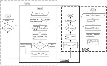
Fig. 3. The flow chart of the improved GNNA, GNMA and GNMNNA.

4. Experiment and analysis

In order to verify the effectiveness and reliability of the improved GA in fault parameter inversion, a numerical example and two real experiments are designed in this paper. The real experiments used the Bodrum-Kos earthquake and Monte Cristo Range earthquake, respectively. In the simulation experiment, GA,NNA, GNNA, GNMA, and GNMNNA were used to invert fault parameters. In order to verify the stability and reliability of different algorithms, the five algorithms were inverted 100 times, respectively, and the fluctuations of the parameters obtained after 100 inversions of different algorithms were recorded. The above algorithm was used to invert the parameters of the Bodrum-Kos earthquake fault, and the inversion was repeated 100 times, and the parameter inversion was recorded. Compare the inversion effects of different algorithms in numerical examples and real experiments, and analyze the problems and possible causes of each algorithm. Finally, use GNMNNA to invert the Monte Cristo Range fault parameters and analyze the earthquake.

4.1. Numerical examples

The simulated fault parameters in this section are as follows:the Poisson's ratio of a given elastic half-space rectangular dislocation model is 0.25,the geometric center of the fault plane is at the origin of the local coordinate system,the center depth of the fault plane is 10 km,the fault length is 22 km,and the width is 12 km,The strike is 120, the dip is 30, the rake is -45, and the slip is 0.8 m. The fault plane is a left-lateral normal fault, as shown in Fig. 4. The projection of the fault plane on the surface is shown in Fig. 4. 48 GPS stations are unevenly distributed around the epicenter location with an area of 38 × 32 km. The Okada [2] model is used to calculate the surface deformation,and random noise is added to the simulated surface displacement. Among them, the standard deviation of the horizontal component is within 1-2 mm, and the standard deviation of the vertical component is within 2-6 mm[37,38].GA,NNA,GNNA,GNMA,and GNMNNA algorithms are used to invert fault parameters.

Fig.4. The simulated GPS surface deformation data.The horizontal components of the GPS data are plotted with black arrows,the solid circles with different sizes represent the vertical components, and the black rectangle represents the fault plane projected on the surface.

One inversion estimates is shown in Table 1.Figs.5 and 6 is the estimation of five algorithms for 100 times repeated inversion.Fig. 7 shows the cumulative calculation time of GA, NNA, and GNMNNA inversion for 100 times.It can be seen from Table 1 that the inversion results of GA and GNMA are similar, and each parameter has a similar deviation with the true value.Among them,the deviation between the strike and rake inverted by GA and the true value is large, and the absolute values of deviation are 0.8614 and 0.6830, respectively. The deviation between the remaining parameters and the true value is small, and the absolute value of the deviation is within 0-0.25.The absolute deviations of the strike and rake retrieved by GNMA from the true value are 0.8488 and 0.6559, respectively. The absolute value of the deviation of the remaining parameters from the true value is between 0 and 0.25.It shows that although the improved GNMA inherits the genetics of GA, it does not improve the situation that tends to fall into local optimality. The estimated value inverted by NNA and GNNA is far from the true value. Among them, the strike, dip, length, and rake inverted by NNA have a large deviation from the true value. The absolute values of the deviations are 3.5311, 3.8602, 6.2811, and 6.2260, respectively. The absolute value of the deviation of the remaining parameters from the true value is within 0-2.5. The strike, dip, and rake inverted by GNNA have large deviations from the true value.The absolute value of the deviation is 3.0482,1.1667,and 3.5973 in sequence.The absolute value of the deviation of the remaining parameters from the true value is within 0-0.6.It can be seen that although the improved GNNA has an increase in inversion precision compared to NNA, its precision is still lower than that of GA and GNMA. In contrast, the fault parameter inversion result of GNMNNA is close to the true value, and the absolute value of the deviation between the estimated parameters of the inversion and the true value is within 0-0.1,and the gap is very small.Compared with GA,its precision is greatly improved,indicating that GNMNNA not only retains the genetic characteristics of GA but also has the characteristics of global optimization.

Fig. 5 shows the 100 times estimations of GA, GNMA, and GNMNNA. Among them, the estimation inverted by GA is represented by a red line, the estimation inverted by GNMA is represented by a blue line, the estimation inverted by GNMNNA is represented by a green line, and the black line represents the true value.The figure shows that the dip,width and rake inverted by GA fluctuate greatly,and the fluctuation range of parameter estimation is 30-30.3、11.7-12、-44.5～-44. Each parameter estimation obtained by GA inversion deviates from the true value as a whole.The strike,dip,length,width and rake obtained by GA inversion are far away from the true value,and the absolute differences are about 1,0.2,0.3,0.2 and 1,respectively.The parameter estimates inverted by GNMA coincide with those inverted by GA, but the fluctuation of parameter estimates inverted by GNMA is smaller than that inverted by GA. Compared with the two, GNMA is more stable.However, the parameter estimates retrieved by GA and GNMA are generally far from the true value. It shows that although GNMA increases the stability of GA to some extent, it does not solve the problem that GA is easy to fall into local optimum.In contrast,the fluctuation range of each parameter inversion by the GNMNNA algorithm is within 0-0.01,and there is almost no fluctuation.The absolute value of the difference between the true value and the parameters estimated by GNMNNA is within 0-0.01. The estimation of some parameters such as depth, slip and X are almost coincident with the true values. This indicates that the calculation results of GNMNNA are stable and reliable.Compared with GA and GNMA, GNMNNA has higher precision and stronger stability.

Fig.6 shows the estimations of 100 repeated inversions of NNA,GNNA and GNMNNA. The estimations of NNA inversion are expressed by gray dotted histogram. The estimations inverted by GNNA are represented by white straight histogram. The estimations inverted by GNMNNA are represented by black straight histogram. The estimated results of GNMNNA shown in Figs. 5 and 6 are the same, but they are shown in different ways. Fig. 5 shows that the inversion result of GNMNNA is very close to the true value.Therefore,Fig.6 no longer lists the true value results separately,but makes a comparative analysis based on the results inverted by GNMNNA. It can be seen that the estimated distribution range of depth,strike,dip,length,width,and rake retrieved by NNA is large,almost uniformly distributed. The distribution ranges of their estimates are 7-14, 110-130, 25-35, 20-35, 10-20, -60～-35. The estimated distribution range of slip, X and Y retrieved by NNA is relatively narrow, but the estimations are also roughly evenly distributed. Their estimation ranges are 0.4-1, -5-5, and 0-5 respectively. It shows that the parameter estimates inverted by NNA fluctuate greatly and the precision is very low.The estimation retrieved by GNNA is roughly similar to the estimation retrieved by NNA. It also has great volatility, and the distribution of parameter estimates is relatively uniform. The distribution range of each parameter retrieved by GNNA is approximately the same as the distribution range of each parameter retrieved by NNA. It shows that GNNA failed to retain GA's heritability,with low accuracy and poor stability. On the other hand, the estimated parameters retrieved by GNMNNA are close to the true value. And from the analysis in Fig. 5, it can be seen that the absolute value of the difference between the true value and the estimated parameters inverted by GNMNNA is within 0-0.01. Therefore, compared with NNA and GNNA, GNMNNA has stronger stability and higher precision.

Fig. 7 shows the cumulative calculation time of GA, NNA and GNMNNA inversion for 100 times. Where, the straight line represents NNA, the point line represents GA, and the dotted line represents GNMNNA. It can be seen that GA has the fastest calculation speed, GNMNNA is the second, and NNA has the longest calculation time.

Table 1 Estimates of the earthquake fault parameters.

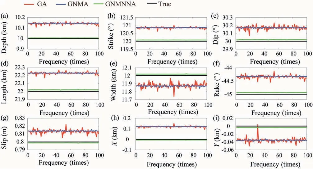
Fig. 5. Estimates of GA, GNMA, and GNMNNA based on left-lateral normal fault deformation field.

Fig. 6. Estimates of NNA, GNNA and GNMNNA based on left-lateral normal fault deformation field.

4.2. MW 6.6 Bodrum-Kos earthquake

On July 20,2017,the M6.6 Bodrum-Kos earthquake occurred on the normal fault in Gokova Bay, Turkey. This paper uses the GPS three-dimensional deformation data in Zhao and Xu [37].The site distribution is shown in Fig.8.There are a total of 20 GPS stations, including 20 horizontal components and 20 vertical components.Numerical examples show that the inversion results of GNMA and GNNA are poor, but the inversion precision of GNMNNA is higher. In order to reduce the computational workload and further verify the reliability and validity of GNMNNA,this section only uses GA, NNA and GNMNNA three algorithms to invert Bodrum-Kos earthquake fault parameters for comparative analysis.

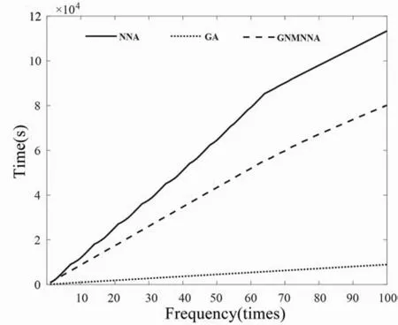
Fig. 7. Cumulative calculation time of GA, NNA and GNMNNA based on left-lateral normal fault deformation.

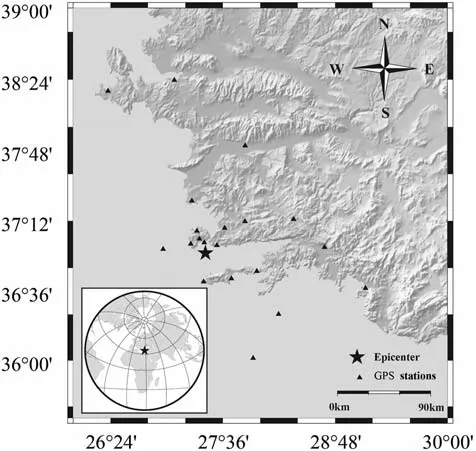
Fig.8. The study area and distribution of GPS stations(Black star is the epicenter.Black triangles are GPS stations of continuous observation).

Table 2 shows the estimation of the Bodrum-Kos earthquake fault parameters obtained by random inversion once.Figs.9 and 10 show the estimation results of the three algorithms repeatedly inverting 100 times.Fig.11 shows the cumulative calculation time of GA,NNA and GNMNNA inversion for 100 times. Table 2 shows that some of the parameter estimates inverted by GA and NNA are quite different from the existing research results.Among them,the absolute values of the difference between the depth,strike,dip,and width retrieved by GA and the existing research results are 1.0967,-2.3073,6.3860,and 1.9854, respectively. The absolute values of the difference between the strike, dip, width, and rake retrieved by NNA and the existing research results are-0.6258,0.4886,-0.5459 and-0.5710,respectively. However, the parameter estimates inverted by GNMNNA have little difference with the existing research results,and the absolute value of the difference between the parameter estimates and the existing research results is within 0-0.2.

Fig.9 shows the estimations of 100 repeated inversions of NNA and GNMNNA. The black point line in the figure represents NNA,the black line represents GNMNNA,and the black dotted represents the results of existing research. It can be seen that the parameter estimates of the strike, dip, width, and rake inverted by NNA represented by the black point line fluctuate greatly, and the fluctuation ranges are 265-267,36.5-37.5,8-9.5,-94～-92.5.In addition,the estimation of each parameter retrieved by NNA is far away from the existing research results as a whole.The fluctuation range of the depth, strike, dip, length, width, rake, slip, X and Y estimations retrieved by GNMNNA are within 0-0.1, and there is almost no fluctuation.And the overall valuation result is close to the existing research results. It shows that the inversion result of GNMNNA is more stable and closer to the existing research results.

Fig.10 shows the estimation results of 100 repeated inversions of GA and GNMNNA. The white dotted histogram in the figure represents GA. The black straight histogram represents GNMNNA.The GNMNNA estimation results used in Figs.9 and 10 are the same data but expressed in different forms.Fig.9 shows that the results of GNMNNA inversion are similar to those of existing studies.Therefore, Fig. 10 no longer lists the existing research results separately,but uses the estimated results retrieved by GNMNNA as a benchmark for comparative analysis.The white dotted histogram shows that the estimated fluctuation range of each parameter retrieved by GA is relatively large. Among them, the estimated ranges of depth, strike, dip, length, width, rake, slip, X and Y are 6-8.5,260-280,25-40,12-24,5-9,-100～-75,1-3,5.5-8,0-4.The parameter estimation distribution takes the form of high middle and low sides. The estimates of depth, dip and width retrieved by GA deviate from the existing research results,and only nearly 20% of the estimates of other parameters are close to the existing research results, and the precision is very low. And Fig. 9 shows that the depth, strike, dip, length, width, rake,slip, X and Y estimated by GNMNNA fluctuate in the range of 0-0.1,and there is almost no fluctuation.And the overall parameter estimation result is close to the existing research results. Therefore, it can be seen that GNMNNA is better than GA in terms of inversion precision and calculation stability.

Table 2 Estimates of the Bodrum-Kos earthquake fault parameters.

Fig. 9. NNA and GNMNNA estimates obtained by repeated inversion 100 times based on the Bodrum-Kos earthquake.

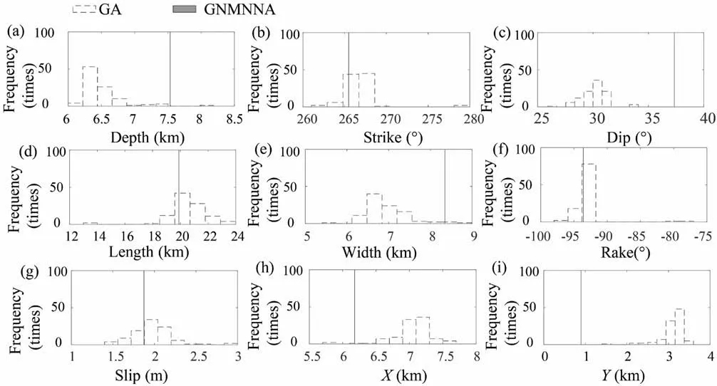
Fig.10. GA and GNMNNA estimates obtained by repeated inversion 100 times based on the Bodrum-Kos earthquake.

Fig.11 shows the cumulative calculation time of GA, NNA and GNMNNA inversion for 100 times. Where, the straight line represents NNA, the point line represents GA, and the dotted line represents GNMNNA. It can be seen that GA has the fastest calculation speed, GNMNNA is the second, and NNA has the longest calculation time.

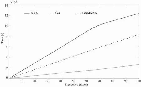
Fig.11. Cumulative calculation time of GA, NNA and GNMNNA based on Bodrum-Kos earthquake.

4.3. MW 6.5 Monte Cristo Range earthquake

On May 15,2020,an M6.5 earthquake occurred 56 km west of Tonopah,Nevada,USA.The earthquake was caused by a strike-slip fault in the shallow crust of the North American plate (the United States Geological Survey (USGS): https://earthquake.usgs.gov/earthquakes/eventpage/nn00725272/executive); the earthquake was selected as the second application of GNMNNA. Zheng et al.[39].used geodetic data to jointly invert the focal mechanism of the Monte Cristo Range earthquake and found that the earthquake caused two fault segments to rupture in different directions.Among them,the east fault is a left-lateral fault,and the west fault contains both left-lateral and normal fault components. And the best fit model shows that the dip of the east fault section is 83,and the dip of the west fault section is 63. This paper uses GPS threedimensional deformation data to reinvert the fault parameters of this earthquake and further test GNMNNA.The distribution of GPS stations is shown in Fig.12. There are 213 GPS stations, including 213 horizontal components and 213 vertical components. The inverted parameter estimates and USGS published results are shown in Table 3.In order to verify the precision of GNMNNA,this paper uses the Monte Carlo (MC) method to sample 100 sets of observation data sets,and invert the 100 sets of data to obtain 100 sets of parameter estimation results.

MC is used to calculate the mean and standard deviation of parameter estimation [40-43]. Firstly, the observation data are sampled s times, and the mean value of parameter estimation is calculated by using the sample:

Fig. 12. The study area and distribution of GPS stations (Black star is the epicenter.Black triangles are GPS stations of continuous observation).

Table 3 Estimates of the Monte Cristo Range earthquake fault parameters.

Table 3 shows the earthquake fault parameters of the Monte Cristo Range retrieved by GNMNNA. It is concluded that the earthquake moment released by this earthquake is 5.21 × 10,the moment magnitude is M6.44,the dip is 66.80,and the rake is -14.42. The fault type is a left-lateral normal fault. The dip inverted by GNMNNA is close to the dip of the west fault at 63inverted by Zheng et al. [39]. And the fault type obtained by GNMNNA is similar to the west fault type. It implies that the earthquake type is mainly left-lateral, and it also illustrates the complexity of the source geometry and fault pattern.And it can be seen from Table 3 that the mean values of the parameters retrieved by GNMNNA are very close to the estimates, but the SD of the inverted strike, dip, length, width, and rake are relatively large, respectively,0.27,1.13,0.61,0.46,and 0.82,and the rest the SD of the parameters are all small, within 0-0.2, indicating that the precision of the inverted parameters is inconsistent when using GNMNNA to invert the fault parameters. Among them, the position, depth and slip parameters of GNMNNA inversion are more stable and accurate, while the inversion parameters of strike, length, width and rake are less stable and accurate.Therefore,when using GNMNNA to invert the source parameters,you can more trust the inverted position, depth and slip parameters. Fig. 13(a) shows the GPS observed deformation value.Fig.13(b) shows the residual value of the simulated deformation value and the observed deformation value. The simulated deformation value is obtained by forwarding calculation using the parameter estimation obtained by GNMNNA. From the perspective of data fitting, the RMS of the east-west, north-south, and vertical components are 1.2964 mm,1.3182 mm, and 4.0114 mm,respectively. It shows that the horizontal RMS is smaller than the vertical RMS.And it can be seen from Fig.13(b)that the horizontal residual is much smaller than the vertical residual.It is considered that the precision of the GPS horizontal observation data is much higher than the vertical observation precision. Therefore, this imbalance of inversion precision may be caused by data. Fig. 14 shows the inversion results of 100 GPS sampling data. It can be seen that the rake has a certain correlation with Y, length, and width. The dip has a certain correlation with Y. There is a certain correlation between length and X and strike. The relationship between the remaining parameters is random.At the same time,it can be seen that the results of each parameter of 100 inversions roughly obey the normal distribution, and the inversion result with only the width tends to the mean distribution. This may be because the fault width estimation is not obtained directly by searching, but using the top depth, bottom depth, and dip are jointly calculated to obtain the fault width. Each inverted parameters contains a certain error, and the cumulative error of different parameters causes the accuracy of the fault width to be low.

5. Conclusion

In this paper,we use special structure of NNA and the local search of NMA to optimize the inversion precision of GA, and proposes a GNMNNA.The purpose is to improve GA and inverse the more stable parametric solution. In the inversion of fault parameters, GA is usually used to invert fault parameters.However, due to the strong heredity of GA operation process, it is difficult to recover once the effective gene is lost, which leads to premature convergence and local optimum of GA.In order to effectively utilize the advantages of GA and avoid its defects, this paper proposes an algorithm with stronger comprehensive ability.In order to fully verify the rationality of the proposed algorithm, this paper designs three combinations,namely, GNNA, GNMA and GNMNNA. Numerical examples show that GNMNNA not only retains the genetic characteristics of GA,but also has the characteristics of global optimization. GNMA inherited the genetic nature of GA,but it did not improve the situation of easily falling into local optimum. Although the parameter inversion precision of GNNA is higher than that of NNA, its precision is still lower than that of GA and GNMA. The Bodrum-Kos earthquake further verifies that GNMNNA is superior to GA and NNA in both inversion stability and calculation precision. GNMNNA was further tested using the Monte Cristo Range earthquake. The precision of GNMNNA is evaluated by the MC method.The experimental results show that the position, depth, and slip parameters retrieved by GNMNNA are more stable and accurate, while the inversion parameters of the direction,length,width,and slip angle are less stable.The accuracy is low. Therefore, when using GNMNNA to invert the source parameters, you can more trust the inverted position, depth and slip parameters.

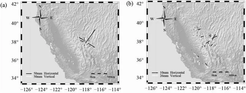
Fig.13. (a) GPS deformation observation; the black arrow is the GPS horizontal deformation observation; the white arrow is the GPS vertical deformation observation. (b) GPS observation value and GNMNNA simulation value residual diagram; the black arrow is the horizontal residual; the white arrow is the vertical residual.

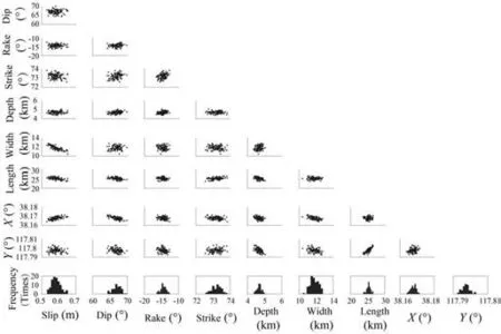
Fig.14. Correlation analysis between seismic source parameters.

Author statement

Leyang Wang: Conceptualization, Methodology, Supervision,Formal analysis, Investigation, Funding acquisition.

Ranran Xu:Conceptualization,Methodology,Software,Writing-Original Draft, Writing-Review & Editing.

Fengbin Yu: Software, Resources.

Con

fl

icts of interest

The authors declare that there is no conflicts of interest.

Acknowledgements

The authors are grateful to all of the anonymous reviewers and editors for their careful review and valuable suggestions, which improved the quality of this paper.This manuscript is supported by the National Natural Science Foundation of China (No.42174011,41874001 and 42174011). Thanks for the discussion with Dr.Guangyu Xu about this paper.Some of the code used in this paper comes from Mathworks website,and some images are drawn using open source software GMT.