A SCR method for uncertainty estimation in geodesy non-linear error propagation: Comparisons and applications

Chunyi Zou , Ho Ding ,b,*, Leyng Wng

a Department of Geophysics, School of Geodesy and Geomatics, Wuhan University, Wuhan 430079, China

b Hubei Luojia Laboratory, Wuhan 430079, China

c Faculty of Geomatics, East China University of Technology, Nanchang 330013, China

Keywords:SCR method Uncertainty estimation Non-linear error propagation Inversion of seismic fault parameter

ABSTRACT We review three derivative-free methods developed for uncertainty estimation of non-linear error propagation, namely, MC (Monte Carlo), SUT (scaled unscented transformation), and SI (sterling interpolation). In order to avoid preset parameters like as these three methods need, we introduce a new method to uncertainty estimation for the first time, namely, SCR (spherical cubature rule), which is no need for setting parameters. By theoretical derivation, we prove that the precision of uncertainty obtained by SCR can reach second-order. We conduct four synthetic experiments, for the first two experiments, the results obtained by SCR are consistent with the other three methods with optimal setting parameters, but SCR is easier to operate than other three methods, which verifies the superiority of SCR in calculating the uncertainty. For the third experiment, real-time calculation is required, so the MC is hardly feasible. For the forth experiment, the SCR is applied to the inversion of seismic fault parameter which is a common problem in geophysics,and we study the sensitivity of surface displacements to fault parameters with errors. Our results show that the uncertainty of the surface displacements is the magnitude of ±10 mm when the fault length contains a variance of 0.01 km2.

1. Introduction

Non-linearity is one of the typical properties in nature. The uncertainty estimation of non-linear error propagation is a quest that has seen continual advances in geodesy and geophysics over the decades [1-4]. Due to the influence of non-linearity, there are no longer unbiasedness and minimal variance of the obtained parameters [5]. A reasonable uncertainty should be given to reflect the true credibility of the result,otherwise the estimations are not convincing[6].For a general non-linear function,the theory of error propagation is mainly used to calculate the uncertainty of the output value. Error propagation can be applied to the linear function form of the non-linear function by the first-order Taylor expansion. A non-linear error propagation formula containing quadratic terms is derived by Ref. [7], which can be used to calculate the uncertainty of second-order precision,but the derivation of the formula is not detailed enough. The generalized variance-covariance propagation law by using the third derivative is established by Ref. [8]. The third-order derivative and above nonlinear error propagation law is applied in GIS (Geographic Information System) by Xue et al. [9]. In the estimation of uncertainty,the precision of first-order is commonly used,and the precision of second-order is slightly higher [10]. The precision of third-order has exceeded the observation level, and it is also difficult to achieve third derivative [11].

The uncertainty can be obtained by first-order Taylor expansion, but the precision is not high enough [12,13]. The secondorder Taylor expansion requires second-order derivation operation, which is tricky when applied to problems with high nonlinear strength (this will be discussed in the second part of this paper). In order to avoid the derivative operation, it is useful to develop derivative-free method for estimating the uncertainty and studying the uncertainty estimation of the general nonlinear function based on the theory of non-linear error propagation.

Some derivative-free methods have been used in geodesy. The Monte Carlo (MC) method has been used to calculate the uncertainty of the total least-squares parameters in Ref. [14]. In geophysics [15], performed the MC to estimate the uncertainty of Love number.It is necessary to add hundreds time of random errors to the result and repeat the experiment to obtain the uncertainty of first-order precision. For the uncertainty of the second-order precision, hundreds of thousands of repeated experiments are required [16,17]. Although today's computer conditions are no longer a bottleneck, the efficiency of hundreds of thousands of repeated experiments is low. In order to improve efficiency of calculation,some scholars introduce other derivative-free methods that differ from MC in the uncertainty calculation of non-linear error propagation [18-21]. In these studies, the SUT (scaled unscented transformation) method is introduced to calculate the uncertainty of the parameter estimation of the non-linear total least-squares [18], and compared with the Taylor expansion, the corresponding precision is improved.Wang and Zhao[19]used the SUT to study the error propagation problem of the general nonlinear function. They treated the non-linear function as an implicit function, and expanded the applicability of the SUT. The SI(sterling interpolation) method was introduced to study the error propagation of non-linear functions [20]. Wang and Zou [21] used SI to calculate the uncertainty of the parameters of the nonlinear inversion. In general, there is no need to repeat hundreds of thousands of experiments like MC to obtain second-order precision uncertainty by SUT, but three parameters need to be set, which makes the process of uncertainty estimation more complicated[22]. Besides, the selection of one parameter is required for SI too.SUT and SI methods were originally used in the system and control field [23-28].

In order to avoid hundreds of thousands of repeated experiments of MC, and preset parameters for the SUT and SI, we introduce another derivative-free method named SCR (spherical cubature rule)method[29,30].There is no need for a large number of repeated experiments and preset parameters.

In Section 2,the error propagation formulas for the general nonlinear function are derived, and we review the MC, SUT and SI methods.In Section 3,the operation process of the SCR method will be described briefly. After then, from the perspective of formula derivation,we prove that the uncertainty of second-order precision can be obtained by SCR. In Section 4, we use three synthetic experiments to compare several methods numerically and verify the correctness of the formula derivation of the SCR.Finally,the SCR is applied to the error propagation of seismic fault parameter inversion.

2. Sampling methods for non-linear error propagation

2.1. Non-linear error propagation

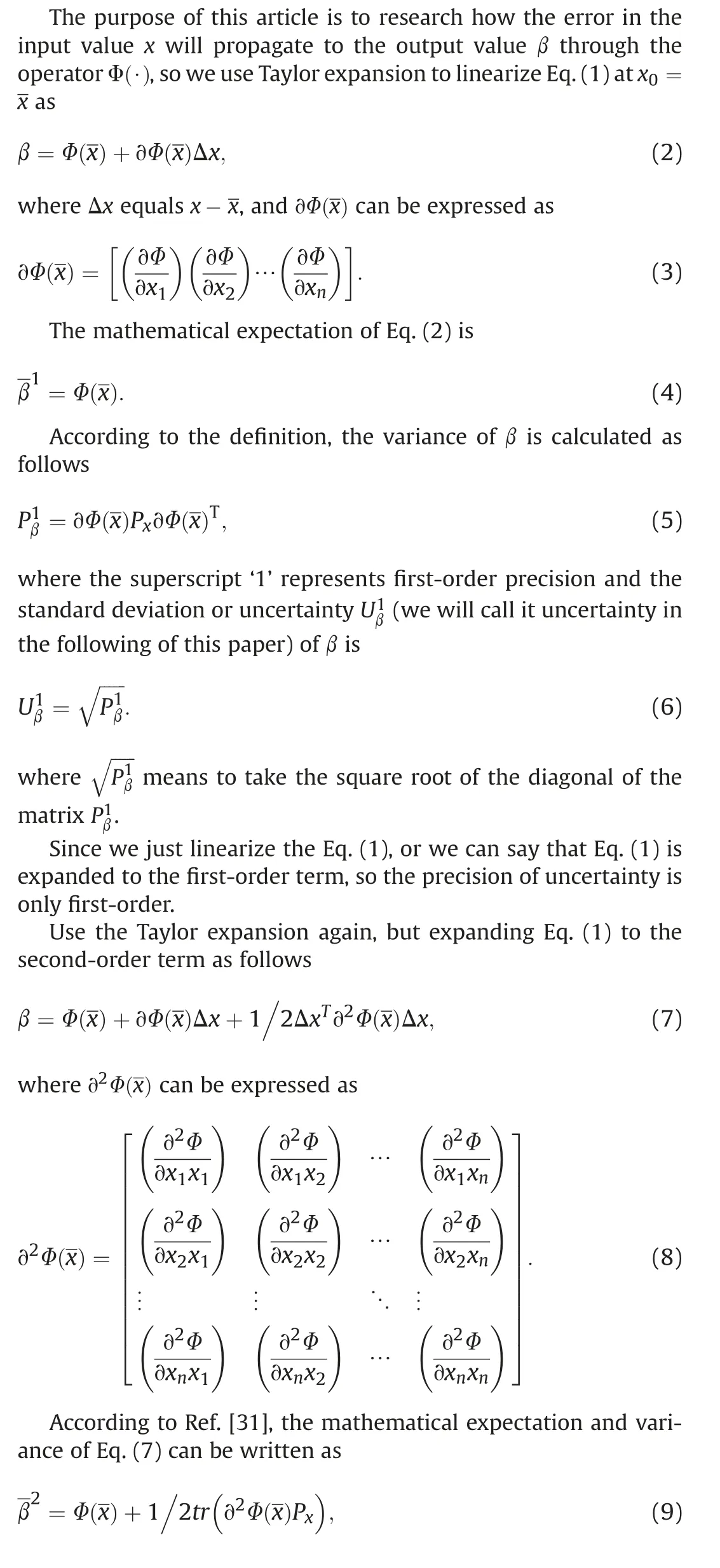
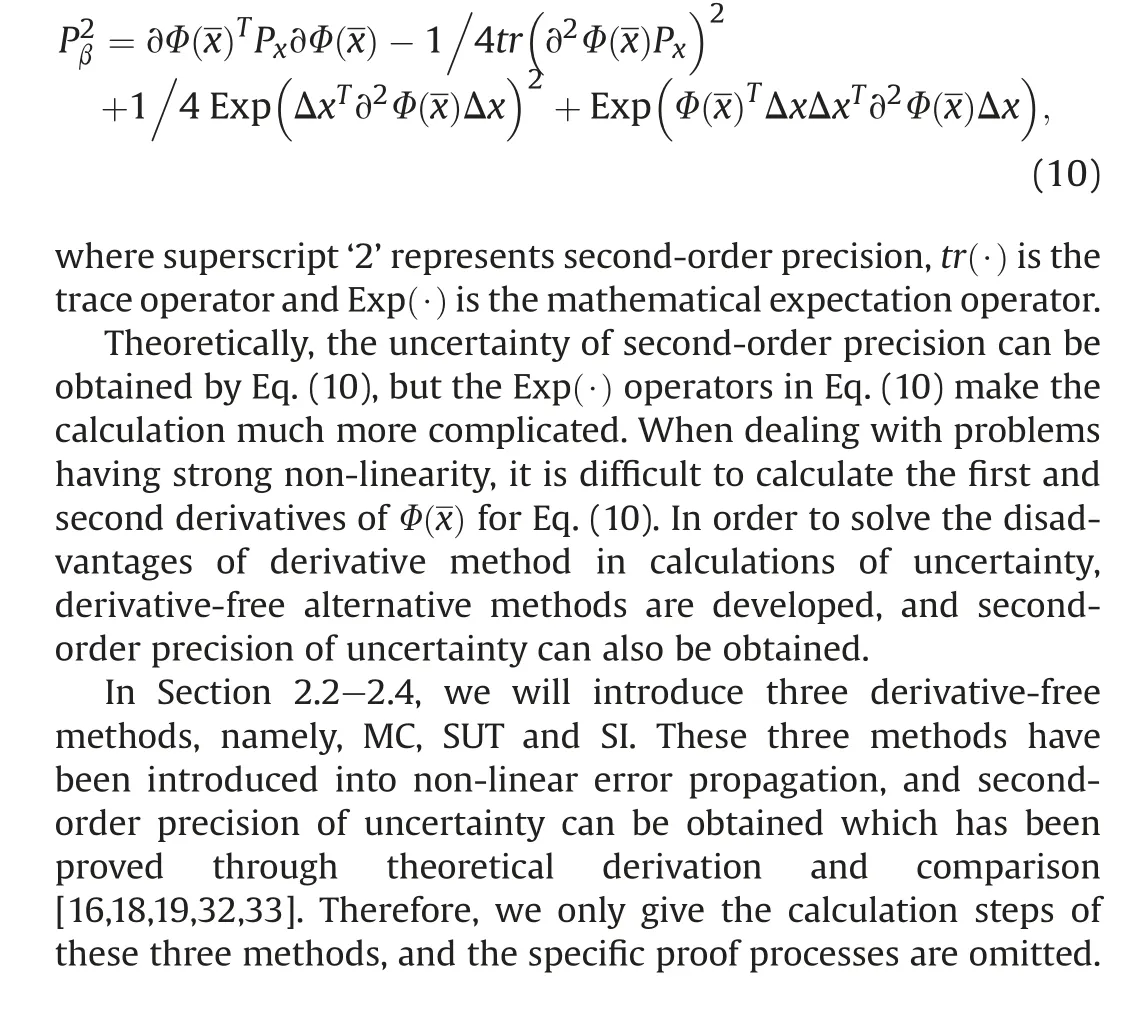
Since we research the uncertainty estimation of non-linear error propagation, a general function is defined as variance of x is P. β is the output value which is obtained by the non-linear operator Φ(·).Since the correlation of the input value is not considered,whether the output value is a scalar or a vector will not affect the precision of the result. For the convenience of the derivation below, we assume that the output parameter β is a scalar.

2.2. Monte Carlo method

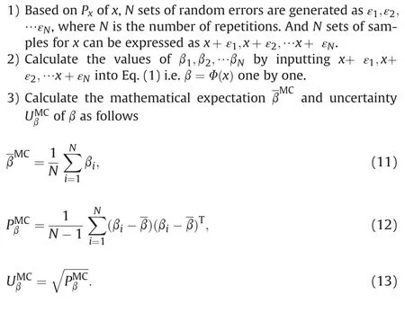
MC method is the most commonly used method in estimating uncertainty, and reasonable uncertainty can be obtained via repeating the experiment for many times. The calculation process can be divided into the following steps [16]:

2.3. SUT method

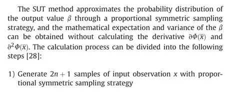
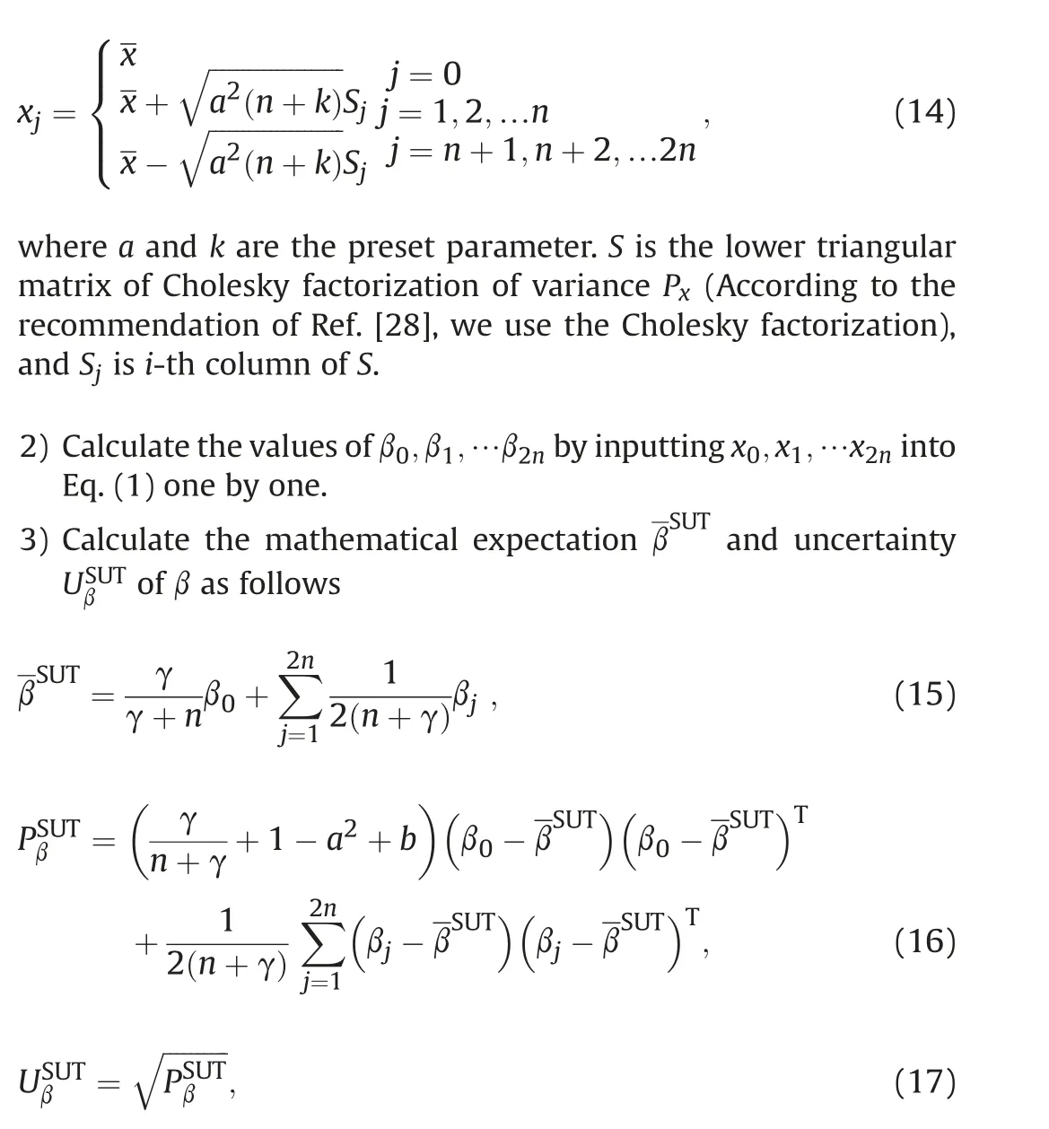
where b in Eq. (16) is another preset parameter of SUT.

It has been proved that the uncertainty calculated by SUT can reach the second-order precision[18,19],and the proof process will not be given here.

2.4. SI method

The SI method is similar to the SUT method to a certain extent.They both proposed by Merwe[28],the calculation steps of SI are as follows.

It has been proved that the uncertainty of SI can reach the second-order precision from theory and experiment[20].It has also been applied to geodesy and geophysics like SUT.

3. SCR sample method for non-linear error propagation

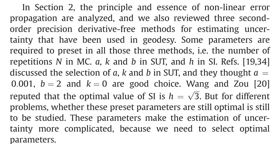
In this section, we will first explain how to carry out the SCR method to non-linear error propagation, and we will theoretically prove that the SCR can get the uncertainty of second-order precision.We will see that there is no parameter in SCR which makes the estimation of uncertainty simple.

3.1. Calculation steps of SCR method

3.2. Proof of second-order precision uncertainty of SCR

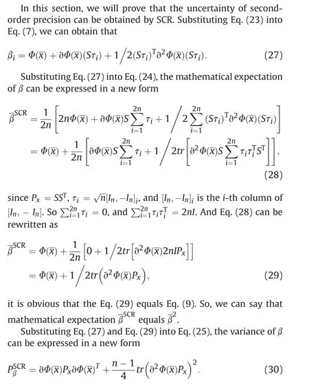
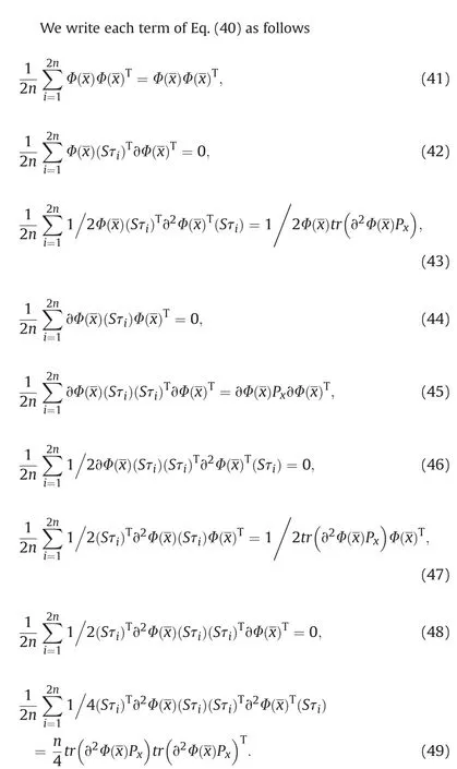
The detailed derivation process of Eq. (30) is listed in the appendix. Eq. (30) cannot be compared with Eq. (10) because there are Exp(·) operators in Eq. (10). But it is easy to find that the precision of Eq. (30) is second-order when n≠1, hence the secondorder precision uncertainty can be obtained by SCR is proved.

4. Experiments

In this section,we use three geodetic experiments to verify the effectiveness of the SCR method,and then apply SCR method to the uncertainty calculation of geophysical inversion.

4.1. Intersection survey

The technique of inferring the plane coordinates of the fixed point by measuring the distance and direction of two known points is called intersection survey. As shown in Fig. 1, the distance between point A and point B is known, and angles α and β are also known. The coordinates of point P can be obtained by Eq. (31).

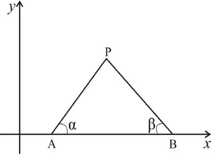
Fig. 1. Schematic depiction of intersection survey. Redrawn according to Fig. 2 of Ref. [20].

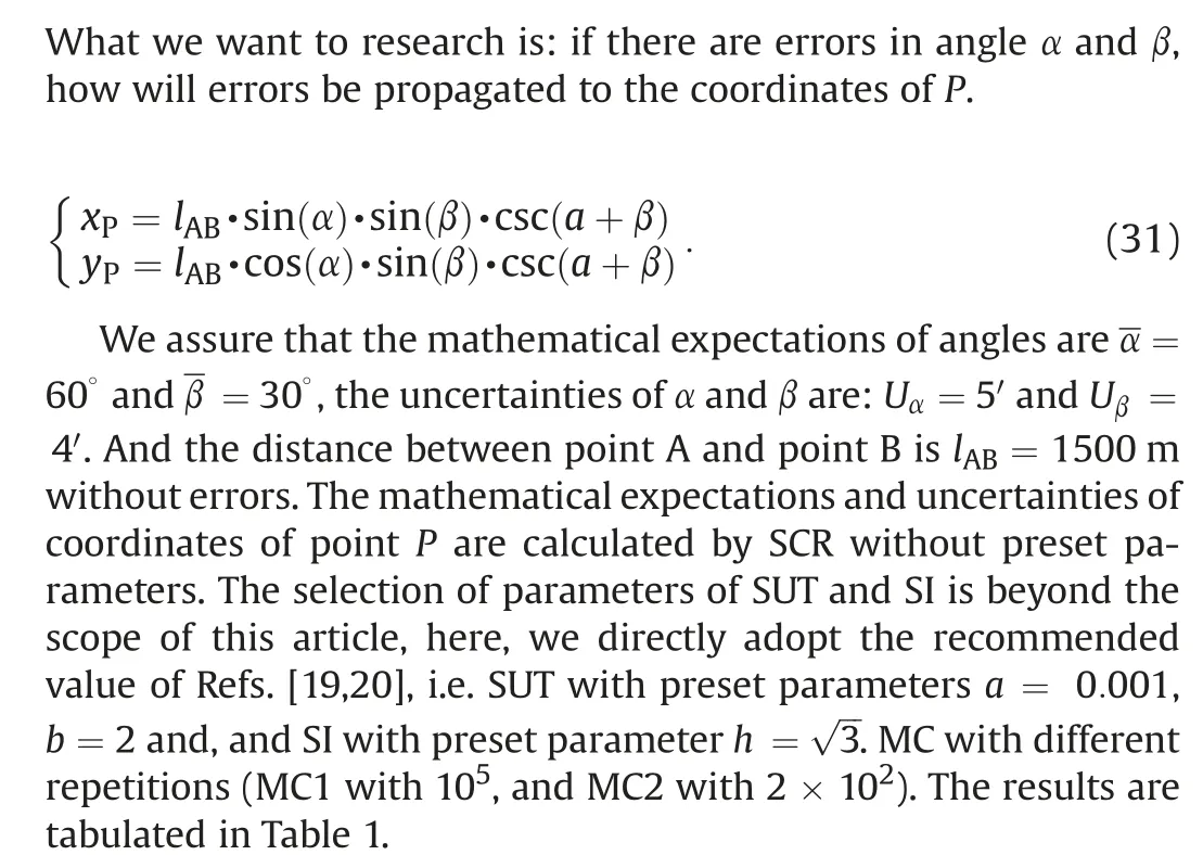
It can be seen from Table 1 that the mathematical expectations and uncertainties calculated by SCR are completely consistent with those from SUT and SI.The differences with the results of MC1 are of the third decimal.This finding shows that the uncertainty of the second-order precision can be obtained in these four solutions.But the difference between MC2 and SCR/SUT/SI/MC1 is of the first decimal,which illustrates that two hundred of repetitions can only get the uncertainty of the first-order precision,it is undesirable.The results of SCR and MC1 are almost the same. Therefore, it can be considered that the SCR method proposed in this paper can achieve the same consequent as MC method with 10repeated experiments. But hundreds of repeated experiments are obviously not enough like MC2.

Table 1 Mathematical expectations and uncertainties of coordinates of point P.

4.2. Polynomial fitting of GPS elevation

The polynomial fitting of GPS elevation is a common model in geodesy [35]. The functional relationship between anomalous elevation and coordinates of plane is non-linear

We will explore how the errors in the plane coordinates propagate to the anomalous elevation.Here,the SCR method is used to calculate the uncertainty of the anomalous elevation,and the SUT,SI,MC1 and MC2 will also be used for comparison.The definitions of MC1 and MC2 are the same as experiment 4.1.We simulated four plane coordinate points, and the priori mathematical expectation and variance for each coordinate are given.Noting that the values of coordinates are given casually, and the values of coordinates does not affect the conclusion of this paper. Therefore the expectations of each coordinate are not important. The variance of the abscissa and ordinate of each point should be equal, which meets the observation requirements.The preset parameters of SUT and SI are same as Section 4.1. Mathematical expectation and variance for each coordinate are tabulated in Table 2. The results of this experiment are tabulated in Table 3.

In the header of Table 3, the mathematical expectation is abbreviated as Exp ζ,and the uncertainty is abbreviated as Unc ζ.Consistent with the conclusions obtained in Section 4.1, the mathematical expectations and uncertainties calculated by SCR are completely consistent with SUT and SI.The difference with the MC1 method is of the third decimal.The uncertainty obtained by MC2 is obviously not up to the second-order precision. This experiment shows that the new sampling method i.e. SCR proposed in this paper is feasible in error propagating of polynomial fitting of GPS elevation.

4.3. Error propagation of GPS baseline vector

High calculation efficiency is not required in previous two experiments. For problems that require calculating uncertainty in real-time, MC method is no longer affordable because the calculation time is too long.

In modern engineering surveys, the combined adjustment of GPS baseline vector networks and terrestrial control networks generally can be accomplished in a two-dimensional coordinate system, and online calculations are required. The spatial rectangular coordinates (X,Y,Z)of each station are calculated by the GPS baseline vector(ΔX,ΔY,ΔZ)between the control point and each station in the GPS network, then the geodetic coordinates(L,B,H) of each station are iteratively obtained. Finally, the plane rectangular coordinates (x,y) of each station are calculated by the positive computation of the Gaussian projection coordinates.

Table 2 Mathematical expectation and variance for each coordinate.

Table 3 Mathematical expectation and uncertainty of each anomalous elevation.

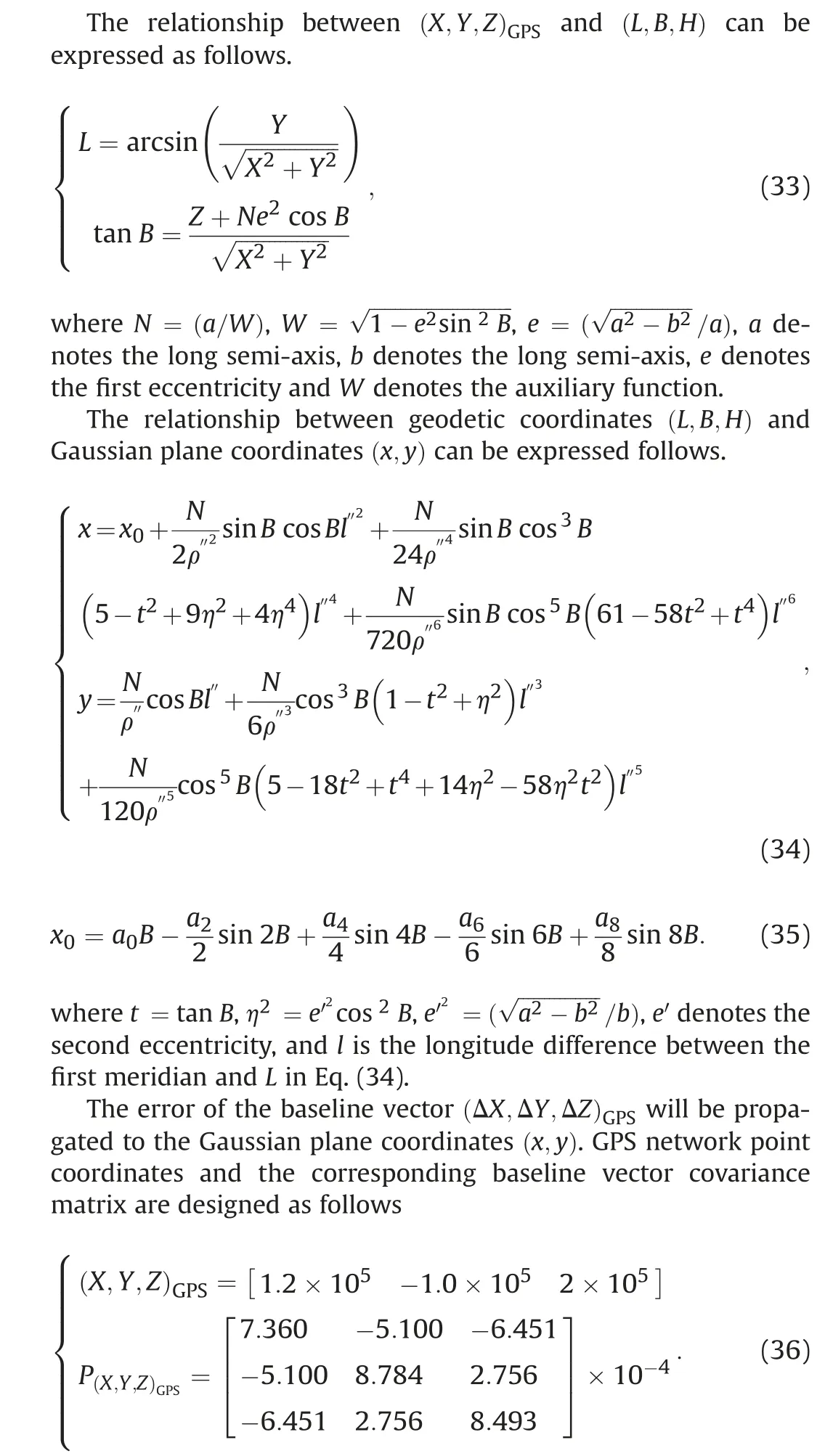
The results of this experiment are tabulated in Table 4. In the header of Table 4, the mathematical expectation is abbreviated asExp x and Exp y, and the uncertainty is abbreviated as Unc x and Unc y.

Table 4 Mathematical expectation and uncertainty of Gaussian plane coordinates (x,y).

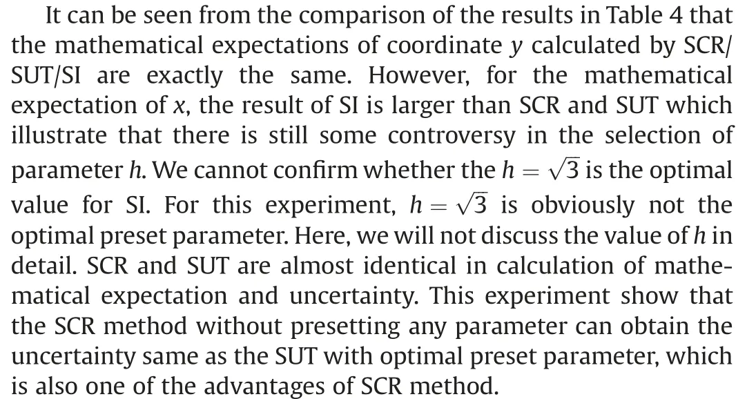
Since the calculation of the error propagation of GPS baseline vector is real-time and has high requirements for calculation efficiency, that MC is hardly feasible.

4.4. Inversion of seismic fault parameters

Inverting seismic parameters with geodetic data is of great significance for studying the mechanism and triggering relationship of earthquakes[36,37].In general,the length,width,depth and inclination angle of a seismic fault are included in the source parameters. The rectangular dislocation model is often used in inversion of seismic fault parameters, it is a complex non-linear model, see Ref. [38] for details. The functional relationship between seismic fault parameters and displacements can be written as follows

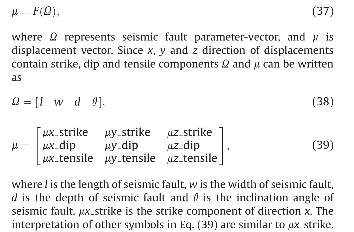
Suppose there are 400 observation points evenly distributed on the ground. We simulate a seismic fault with length of l = 10 km,width of w = 6 km, depth of d = 6 km and inclination angle of θ = 40under the ground. The schematic depiction of the seismic fault is plotted in Fig.2.We use the rectangular dislocation model to calculate the displacements of the observation points. The displacements are shown in Fig. 3. It can be found that the displacements of the observation points have reached the level of 100 mm.

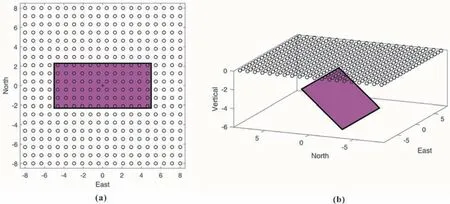
Fig.2. Schematic depiction of the seismic fault.(a)Vertical view of the seismic fault,the purple rectangle is the projection of the seismic fault on the ground,‘+’is the projection of the center of the seismic fault on the ground. (b) Lateral view of the seismic fault.

If there are errors in the fault parameters, the errors will be propagated into the displacements through the non-linear rectangular dislocation model. The uncertainties of the seismic fault parameters are calculated by Ref. [21], but there are few papers to research the uncertainties of the displacements.In this experiment,we will only use the SCR method to calculate the uncertainties of displacements, which is an application of SCR in geophysics.

In order to study the influence of uncertainties in a single fault parameter on displacements, it is supposed the variance of length of seismic fault is 0.01 km.The uncertainties of the displacements of the observation points is plotted in Fig. 4.

From Fig. 4, we can find that the strike component is not sensitive to the uncertainty in the length of seismic fault.In the west and north directions, errors almost not be propagated to the displacements. The largest uncertainty exists in the dip and tensile components in the z direction, and the value is larger than the other components in one order of magnitude. This may be related to the distribution of seismic fault,which is beyond the scope of this paper and will not be discussed here.The SCR method is applied to study the sensitivity of displacements to parameters of seismic fault which is helpful for understanding the complexity of earthquakes.

Fig. 3. Displacements of the observation points.

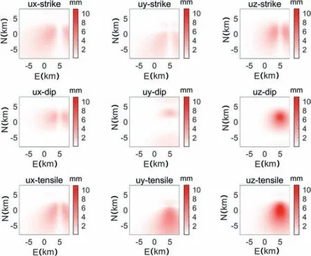
Fig. 4. Uncertainties of displacements of the observation points calculated by SCR method.

5.Conclusions

We briefly explain the error propagation formulas of the general non-linear function, which has limited applicability due to the requirement of derivative. Four derivative-free sampling methods are reviewed, namely MC, SUT, SI and SCR. Among them, SCR is introduced into the non-linear error propagation for the first time.We prove that the uncertainty of second-order precision can be obtained by SCR.

We use the SCR in four synthetic experiments. In the first two experiments, we calculated the uncertainties for the coordinates of a fixed point in the intersection survey and the uncertainty of the anomalous elevation in the polynomial fitting of GPS elevation. The results obtained by SCR are same as those obtained from SUT, SI and MC1. We also show that the second-order precision uncertainty can't be obtained by repeated MC experiments for hundreds of times. Compared with other methods, the advantage of the SCR method proposed in this study is that there is no preset parameter, which simplifies the process of determining uncertainty. The third synthesis experimental, MC method is no longer applicable, results show that the SCR method without presetting any parameter can obtain the uncertainty consistent with the optimal parameters of SUT, but the result of SI is significantly larger than SCR and SUT which illustrates that SCR method may be better when the preset parameters of SUT and SI are not optimal.

In the last experiment, we apply SCR to the parameter inversion of seismic fault, and calculate the uncertainties of displacements when there are errors in length of seismic fault.The results show that when the fault length contains errors with a variance of 0.01 km, the level of uncertainty is about 10 mm.The sensitivity of uncertainty of displacement to other seismic fault parameters is worth studying in future. How to apply SCR method to the measured data is the next problem worth studying in future.

Author statement

Both authors reviewed the results and approved the final version of the manuscript.We confirm that this work is original and has not been published elsewhere nor is it currently under consideration for publication elsewhere.

Con

fl

icts of interest

The authors declare that there is no conflicts of interest.

Acknowledgments

We thank Yingwen Zhao for code of rectangular dislocation model, and Kunpeng Shi for help in plotting pictures. This work is supported by the National Natural Science Foundation of China(41721003, 41974022, 41774024, 41874001). Open Research Fund Program of the Key Laboratory of Geospace Environment and Geodesy, Ministry of Education, China(20-02-05).

Appendix. The detailed derivation process of Eq. (30)