Adaptive neuro fuzzy inference system for predicting sub-daily Zenith Wet Delay

Jareer Mohammed

Civil Engineering Department, Wasit University, Kut, Iraq

Keywords:ANFIS ZWD Weather forecasting GNSS meteorology

ABSTRACT In recent years, the focus of tropospheric studies has evolved to GNSS meteorology and weather forecasting.The Zenith Wet Delay(ZWD),which might be assembled to the Integrated Water Vapour(IWV),is an essential component of the tropospheric delay.Acquiring predicted the ZWD with the required level of accuracy is crucial for weather forecasting. The scope of this study is to use the adaptive neural fuzzy inference system (ANFIS) to predict the ZWD for the following six-hour epoch based exclusively on the present the ZWD value. It was developed and verified using 505 geographically and internationally distributed stations which were used for training and testing from 2008 to 2019.It was assessed based on two criteria. First, the correlation coefficient (R) values were found to be more than 0.8 in 98% of the stations, including those with highest and lowest latitudes, and the remaining 2% of stations located in coastal areas. Second, the Root Mean Square Error (RMSE) values of the differences between the predicted and the actual ZWD were considered to be the more important finding of the study.That is,99.21%of the 505 stations had the RMSE values equal to or less than 3 cm,with only 4 stations having the RMSE values higher (0.2 mm) than 3 cm. Since the results of this study achieved the required degree of accuracy from the predicted ZWD to be utilized in weather forecasting, they may also be beneficial for GNSS meteorology.

1. Introduction

The Zenith Total Delay(ZTD)represents the delay which is from the tropospheric effects on GNSS signal propagation. It has to be computed by following different strategies through PPP[1]or GNSS Network adjustment. It consisted of two components, which are Zenith Hydrostatic Delay (ZHD) and Zenith Wet Delay (ZWD) [2].The ZHD could be computed based on the available meteorological data and it is very predictable. For example, it can be computed using tropospheric models such as Leandro, Langley [3], Boehm,Niell[4]and Saastamoinen[5]or possibly through the processing as an unknown in the Extended Kalman Filter[6].Differently,the ZWD has been considered as non-predictive component and has to be computed through the PPP processing as an unknown due to the temporal and spatial dramatic changing[7].

With the increasing density of meteorological stations,and thus the number of time series data increased,researchers were able to investigate various methodologies for dealing with these data such as machine learning [8], which had been used for solar radiation prediction in Shamshirband, Mohammadi [9] or for forecasting geomagnetic storms in Andriyas and Andriyas [10]. Petkoviˊc,Shamshirband [11] utilized Support Vector Regression (SVR) to predict the modulation transfer function while Shamshirband,Petkoviˊc [12] employed SVR to forecast wind turbine response torque.In addition,Shamshirband,Petkovic[13]performed SVR to increase sensor fusion tracking capabilities, while Joviˊc, Danesh[14] used SVR to estimate robotic finger contact forces.

One of the important machine learning methods is the Adaptive Neuro Fuzzy Interface System(ANFIS) which was proposed by Jang[15].ANFIS has been used in Wind Turbine Systems,for example,the wind speed estimation [16,17], the maximum output power maintaining[18],and wind farm efficiency estimation based on turbine number[19].Petkoviˊc,Nikoliˊc[20]later utilized ANN to predict wind speed fluctuations. It also has been used to estimate friction factors in pipelines [21] and to aid in the underwater laser process[22]. It has further been proposed for determining the relationship between finger contact forces and sensors’stresses[23]and selecting the most convincing precipitation concentration index in Serbia based on precipitation readings [24]. It used in education [25] and distant learning application [26]. Milovanˇceviˊc, Nikoliˊc [27]utilized ANFIS to monitor pumping aggregate vibrations, while Petkovic,Petkoviˊc[28]used it to forecast biomass oxidation.Lakovic,Khan[29]projected better biomass heating values,whereas Kuzman,Petkoviˊc[30] found the best fertilizer parameters and Miliˊc, Petkoviˊc [31]found the highest fatty acid methyl ester and exergy efficiency in situ transesterification process.

For water resources, it has been adopted by several studies[32-35].Mellit,Arab[32]applied the ANFIS to a 9-year time series of mean sunshine time and air temperature to predict the total solar radiation and showed that it could forecast the solar radiation in Algeria with 98% correlation coefficient. Later, Sumithira and Nirmal Kumar [33] utilized ANFIS to predict the monthly global solar radiation in Tamilnadu, arguing that ANFIS is a reliable prediction approach.It has also been used to forecast rainfall,as Talei,Chua[34]evaluated several ANFIS models of rainfall and discharges and concluded that the better model for the non-sequential time series of rainfall was the superior model. When it comes to air pollution, Zeinalnezhad and Chofreh [35] employed ANFIS and discovered that it might be predicted with a mean absolute error of 15%.Further,Feizi,Voosoghi[36]used it to model the Total Electron Content (TEC) for the TEC time series from 29 GPS stations in Iran and found that it could reach an accuracy of about 1.5 TECU while Akyilmaz and Arslan [37] used it to calculate the time lag of the ionosphere. In comparison to Artificial Neural Network (ANN) or Global Ionospheric Model(GIM),Ghaffari Razin and Voosoghi[38]applied ANFIS with Principal Component Analysis (PCA) for the ionospheric time series for one station in Iran and ended up finding that it could provide accuracy of 1-4.72 TECU in the temporal modelling of TEC. Sun, Wang [39] hypothesized that a hybrid combination of ANFIS and Particle Swarm Optimization (PSO)might overcome the restricted positioning accuracy by enabling the categorization of the GNSS signal type.

While the ZWD is most significant for the GNSS accuracy, it is also necessary for weather forecasting, as Hassanli and Rahimzadegan [40], Sangiorgio, Barindelli [41], and Zhao, Liu [42] demonstrated. Different approaches have been attempted to forecast the ZWD such as Katsougiannopoulos and Pikridas [43] who utilized MLP (multi-layer perceptron) to predict ZTD for 6 EUREF stations and discovered that the predicted the ZTD might be as accurate as 3 cm. Ding, Hu [44] applied a back propagation neural network to analyse the residuals between Saastamoinen model and the computed tropospheric delay based on GNSS observations and the meteorological data from 11 International GNSS Service (IGS) stations, resulting in a new tropospheric model (ISAAS) that is comparable to real time tropospheric delay. Similarly, Selbesoglu [45]used back propagation neural network to predict the ZWD from 40 stations in Austria,where the inputs are the location of the stations and the meteorological data, to interpolate the ZWD for missing stations and noticed that it can interpolate the ZWD with a 6 mm accuracy. While Zheng, Hu [46] utilized ANFIS to construct a local prediction model of the ZTD using meteorological data with the Hopefield Model [47], they proved that their model outperformed the Hopefield model alone.

Suparta and Alhasa [48] compared ANFIS with ANN for computing the PWV values based on surface meteorological data and revealed that ANFIS has better performance and could be used to predict PWV, whereas Yue and Ye [49] estimated PWV using ANN and discovered that ANN might provide a good estimation.Suparta and Alhasa [50] used ANFIS to estimate Zenith Path Delay(ZPD)from combined pressure,relative humidity and temperature,which could then be mapped to ZTD using Niell [51]. They compared their results to those of the individual combinations and concluded that using all meteorological data mentioned was better compared to the various combinations of the individual ones.However, they did not test the amount of error that might be obtained between the predicted and the real ZPD, and they only utilized 5 selected Antarctica sites.

It is well-known that no worldwide or temporal research has been conducted for forecasting ZWD by ANFIS without the use of additional meteorological data.The hypothesis that will be tested is the possibility of using ANFIS as a prediction tool for the ZWD on a global scale without relying on the meteorological data, and investigating the obtained level of accuracy based on a monthly and sub-daily basis and comparing them to the required accuracy from published papers and COST Action report that specifies the target required accuracy of ZWD for numerical weather prediction(NWP).The findings should make an important contribution to the field of weather forecasting and the GNSS meteorology.

2. The study area and datasets

The availability of meteorological stations and the density of stations with 10 years of data allow these data to be used for processing.When analysing the ANFIS technique,it is critical to study the method globally and for as long time as feasible in order to make a considerably reliable judgment regarding the appropriateness.As a result,the data from Landskron and Bohm[52],which comprised of various meteorological data such as ZWD and ZHD as well as other meteorological data,were analysed and counted to be 555 stations. Many researchers rely on the availability of this data[6,8,57-66].

Beginning on January 1, 2008, the data were accessible in 6-h temporal resolutions of 00:00, 06:00, 12:00, and 18:00 UTC. The data has been chosen to cover a period of 12 years from the beginning date to the end date. All stations (555 in total) were verified to ensure that they had complete and continuous recordings for the selected time period.However,50 of these stations were discovered to have missing data,resulting in only 505 stations could be used for this study. As shown in Fig.1, these stations are dispersed globally, in addition the geographical, height, and latitude distribution of the stations were taken into account.

The ALRT,MOIU and SCTB stations were selected as examples in Fig.2 to demonstrate the time series of the ZWD form 2008 to the end of 2019 as highest, middle and lowest latitude.

3. Methodology

3.1. Adaptive network based fuzzy inference system (ANFIS)

Zadeh [53] introduced fuzzy set theory and fuzzy logic, which were prepared for soft computing methods inspired by the artificial intelligence.The adaptive network-based fuzzy interference system(ANFIS) is a type of artificial neural network (ANN). Sugeno fuzzy models serve as the foundation for this fuzzy interference system.Both neural network and fuzzy logic concepts must be integrated in order to take full advantage of both in a single framework.Since the inference systems follow a set of fuzzy if-then rules, it has the ability of learning and could be approximated to a nonlinear function, for example.

Fig.1. a)The distribution of 505 stations used in this study with b) their height and latitude distribution.

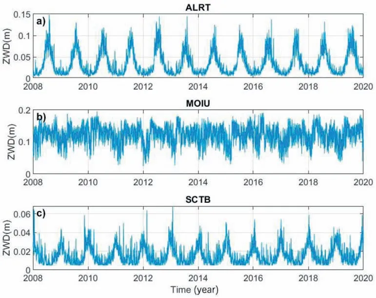
Fig. 2. Time series with 6-h time resolution of ZWD for ALRT (a), MOIU (b) and SCTB (c) stations as highest, middle, and lowest latitude for the period 2008 till the end of 2019.

In this study, ANFIS was used instead of FIS because the latter couldbeadoptedintheframeofanadaptivenetworkandtoavoidthe design and selection of the membership function, as suggested by Alsadik,Gerke[54]since ANFIS computed the membership functions automatically using grid partitioning or clustering techniques.

In this procedure, the ANFIS setting was utilized to predict the ZWD at time t+6 h from ZWD at time t. It was chosen as one for producing ZWD t+1 from ZWD t for the delay.The total amount of data used in this processing was 12 years, resulting in 17,531 observations for a 6-h resolution time.The data was divided into two parts.The first part was chosen to be 75%of the data for the training part, from 1/1/2008 till 31/12/2016, for a total of 13,148 of 17,531 data.This is the train input,which is represented as[zwdzwdzwd…zwd].While the train targets are(13,148*1)which is[zwd tr 1 zwd tr 2 zwd…zwd].The second part contains the remaining 25%of data for each station from 1/1/2017 till 31/12/2019.To test the methodology,the test input will be(4383*1),and the test targets will be (4383*1).

The number of clusters was set to 10,Partition matrix exponent was set to 2,and the minimum number of iterations was set to 100,with chosen minimum improvement threshold to be 1×10[55].The method name used was “Sugeno” [56] and method Probabilistic (prod)or method Probabilistic-OR (probor) of fuzzified input values was employed [57]. While the FIS implication method is product “prod”, the FIS aggregation method is summation per individual element “sum”, and the FIS Defuzzification Method is“weight average” [58].

The flowing options were set to train ANFIS:Maximum Number of Epochs: ‘100’, Error Goal: ‘0’, Initial Step Size: ‘0.01’, Step Size Decrease Rate: ‘0.9’, Step Size Increase Rate: ‘1.1’ and the Optimization Method = 1(1: Hybrid) [59].

The processing will be carried out iteratively for each station independently.The results of using each station from the described datasets were summarized based on two statistical criteria.

4. Results and discussion

The ZWD from each station of the completely recorded 505 stations specified in section 2 in each epoch from 2008 to the end of 2019, was employed for the processing as an input for the ANFIS structure. The predicted ZWD for each station at each epoch was the output.Following all settings in section 3.1,the processing was done for each station independently. Rather than analysing the network itself, it is crucial to evaluate the network's potential for forecasting the real ZWD after training it using data from the beginning of 2008 to the end of 2016. This should be followed in order to make an informed conclusion regarding the method's suitability for delivering ZWD with sufficient accuracy to meet the requirements for weather forecasting. As a result, the testing data from the beginning of 2017 to the end of 2019 were used in the testing part after the network was trained. This has been done for each station separately, which means that each station has been utilized independently. The predicted ZWD was stored so that it could be analysed and compared with the real ZWD.As an example,Fig. 3 shows the time series of the real and the predicted ZWD for ALRT, MOIU and SCTB stations. These stations represented the highest, middle, and lowest latitudes of the dataset.

Fig. 3 illustrates that the predicted ZWD compares well to the actual ZWD, which may be attributed to the use of ANFIS for predicting ZWD.Two characteristics have been chosen for statistically comparing and analysing the predicted ZWD with the actual ZWD in order to investigate the accuracy level of the predicted ZWD,they are R values and RMSE.

4.1. R values analysis

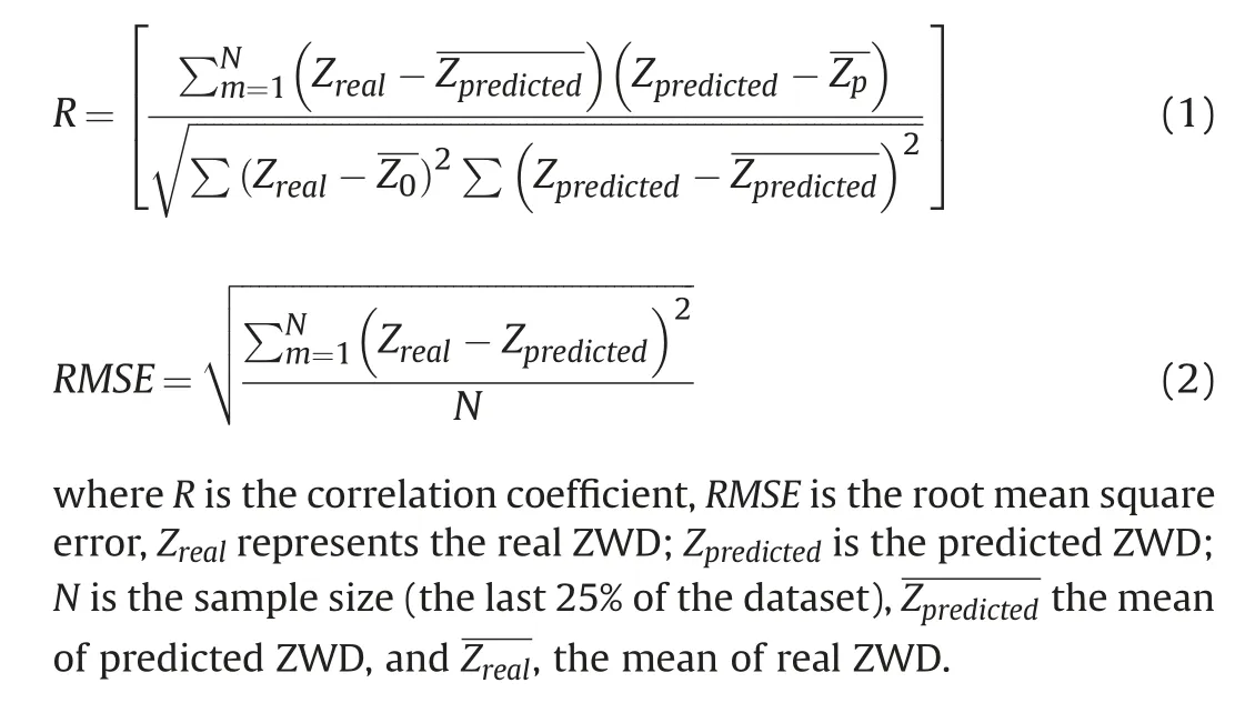
The correlation coefficient (R) has been applied to analyse the correlation between the predicted and the actual ZWD to better understand the possible degree of correlation generated by this approach. The R values for all the 505 stations in this study have been calculated and presented in Fig.4. To understand if there are failed stations in this statistical criterion, the R values of all the stations utilized in the processing were computed.

Fig. 4 clearly shows that R values have been categorized into three groups:stations with R values more than 0.9(green),stations with values between 0.8 and 0.9 (blue), and lastly stations with a correlation less than 0.8 (red).

For this statistical criterion,85%of the stations have the R value over 0.9, which makes them optimal in terms of this statistical criterion. It is important to note that all the stations located at the highest and lowest latitudes show a strong correlation between the predicted and the real value of the ZWD.While the stations with R values between 0.8 and 0.9 were identified to be 13%.KRGG,KERG,MAC1, CZTG, FALK, PARC, RGDG and RIO2 were the remaining stations(2%)that might be considered to have the lowest R values.The fact that these stations have low R values might be attributed to their coastal location.This might occur in these locations where the ZWD accuracy is lower than in inland areas,as reported by Zhang,Li[60] and Ziskin Ziv, Yair [61].

Although the majority of the stations has excellent R values and has satisfied this criterion,it is necessary to examine the accuracy of the differences between the predicted ZWD and the real ZWD of the testing data.

4.2. RMSE analysis

The overall accuracy of ANFIS for predicting ZWD may be evaluated by comparing the real values of the ZWD with those generated from the ANFIS processing as predicted ZWD values for each epoch at each station.As a result,it is essential to consider the differences between the predicted ZWD and the real ZWD values.The RMSE value for each station in the data processing was computed and summarized in Fig. 5.

According to Fig.5 and the analysis of the RMSE values,8.91%of the total stations(505 stations)have excellent RMSE values(≤1 cm accuracy), with 76.44% of the total stations having RMSE values ≤2 cm. The most significant result is that 99.21% of 505 stations have RMSE values ≤3 cm. It is worth emphasizing that these RMSE values were calculated for the entire period from the beginning of 2017 to the end of 2019. Since these numbers reflect the testing period, which is 3 years of data with a 6-h temporal resolution,this may be regarded as a site potential for the degree of accuracy to forecast the ZWD.

This discovery outperforms the 72-82% overall accuracy achieved by Sangiorgio, Barindelli [41].

It is critical to obtain an accurate ZWD within 30 mm precision for computing a reliable IWV from ZWD, as recommended by Ahmed, Teferle [62]. It also consisted with the user requirement for GNSS meteorology from the COST Action 716 [63], which suggested that the needed degree of ZWD accuracy was 30 mm to be appropriate for the present Numerical Weather Prediction(NWP).The accuracy level in this study clearly meets the degree of accuracy necessary for providing accurate ZWD values for global weather forecasting. Furthermore, these results are better compared to those obtained by Su and Jin [64] and equivalent to those obtained by Sun, Zhang [65], since just 4 stations (out of 505) (‘GODE’, ‘GODZ’, ‘GODN’, ‘USNO’) had RMSE larger (0.2 mm)than 3 cm. The level of accuracy achieved by this work will be essential for weather forecasting as well as GNSS meteorology. It is important for the latter when these values are utilized as initial values for the ZWD from VMF1 as in Webb, Penna [66] and Mohammed, Moore [67].

Fig.3. Time series for the predicted and real ZWD for ALRT(a)(highest latitude),MOIU(b)(middle latitude)and SCTB(c)(lowest latitude)for the testing data from 2007 till the end of 2019.

Fig. 4. Correlation of coefficient between the predicted and the real ZWD of 505 stations for the testing data from 2007 till the end of 2019.

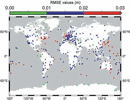
Fig. 5. RMSE values for the differences between the predicted and the real ZWD for the testing data of the 505 stations from 2007 till the end of 2019.

It is well known that the ZWD is considered to be associated with the height and latitude of the stations.As a result,it is vital to continue our investigation and comprehend how these RMSE values may be presented in relation to the station's height or latitude. Thus, Fig. 6 summarizes the RMSE values of the differences between the predicted and real ZWD for the 3 years testing data(2017-2019)with respect to the station's height and latitude.

Fig. 6 shows that there is a notable trend in the correlation between the RMSE values and the height of the stations,implying that as the height of the stations increases, so will the accuracy of the predicted ZWD.This conclusion was similar to that of Jin,Park[68].This can also be shown in Fig. 6 (a), where the same stations with RMSE values larger than 2.5 cm are found at symmetrical latitudes.This figure is comparable with the figure of Mohammed[8],which takes into account the improved accuracy that might be achieved for latitudes larger than 60and less than -60.

4.2.1. RMSE values based on monthly time resolution

It is essential to consider the degree of accuracy of the results obtained based on various weather sessions. As a result, it is important to conduct an analysis to understand the effectiveness of the monthly RMSE values throughout the whole testing period. It will be expressed by computing the RMSE from the differences between the predicted and real ZWD values for the entire testing data based on a monthly basis.From the beginning of 2017 to the end of 2019, these monthly RMSE values were generated for the testing data, and have been collected and shown in Fig. 7.

The RMSE values vary monthly, as shown in Fig. 7. Almost majority of the stations have RMSE values of less than 3 cm (green),which is the required accuracy for the ZWD to be used for weather forecasting.While the remaining stations with RMSE values larger than 3 cm(red)are not regarded to have failed the test all year.As a result, these stations might be classified as seasonally dependent.This was clearly observed from the stations in the northern hemisphere throughout the months 1 (January), 2 (February) and 3(March).

4.2.2. RMSE values based on six-hour time resolution

When I was superintendent1 of schools in Palo Alto, California, Polly Tyner, the president of our board of trustees（）, wrote a letter that was printed in the Palo Alto Times. Polly s son, Jim, had great difficulty in school. He was classified as educationally handicapped and required a great deal of patience on the part of his parents and teachers. But Jim was a happy kid with a great smile that lit up the room. His parents acknowledged his academic difficulties, but always tried to help him see his strengths so that he could walk with pride. Shortly after Jim finished high school, he was killed in a motorcycle accident. After his death, his mother submitted this letter to the newspaper.

Fig. 6. RMSE values for the differences between predicted and real ZWD for 3 years testing data relative to the height (a) and latitude (b) of the station.

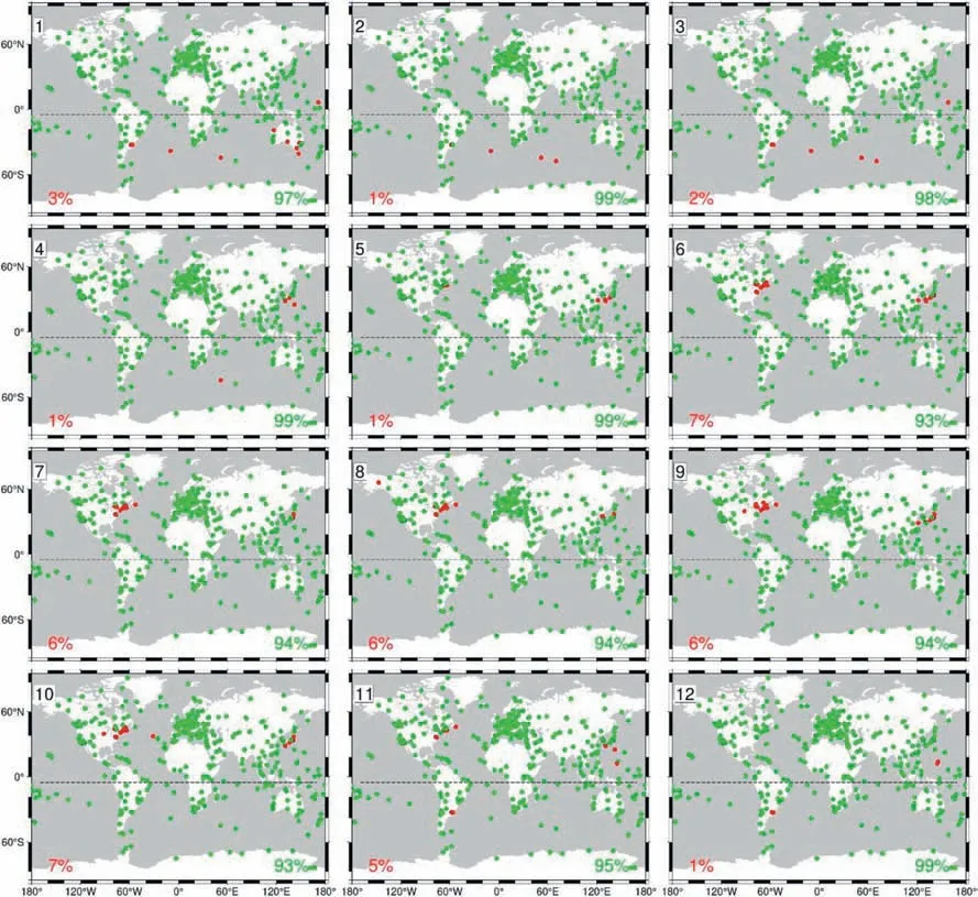
Fig.7. Monthly(January-December)RMSE values for all the 505 stations of the testing data(2017-2019),where RMSE equal or less than 3 cm(green),or greater than 3 cm(red).

Given that our dataset contains 4 ZWD values each day, it is essential to realise the daily behaviour of the acquired accuracy from the predicted ZWD utilizing ANFIS.As a result,the differences between the predicted and the observed ZWD values of each station have been computed using a 6-h time resolution,implying that the RMSE values have been computed for 00:00,06:00,12:00 and 18:00 UTC at each station over 3 years of testing data and are summarized in Fig. 8.

Fig.8 demonstrates that the RMSE values are outstanding given the number of data sets used. Only the stations in red have been determined to fail the RMSE criterion on a 6-h time resolution basis. These stations will not be investigated further for two reasons: first, because of the large number of successful stations, and second, because they are located in coastal areas [61].

4.3. Categorization of the mean values

In addition to the RMSE analysis, the differences between the predicted and real ZWD should be examined to determine any bias.As a consequence, for the 2017-2019 period, mean values were computed as the difference between the predicted and the real ZWD values for each station and visualized in Fig.9 using only the positive and negative classification of the mean values.

Fig. 9 shows that these values are seasonally correlated, since all the stations(in months:11,12,1,2 and 3,and some months are the majority) have negative mean values for the northern hemisphere stations. on the opposite, the following months are represented by the mean values of the stations in the southern hemisphere.Fig.10 shows the negative and positive classification of the mean values between the predicted and real ZWD for the 6-h time resolution.

Although the ZWD is rapidly changing spatially and temporally as Bevis, Businger [2] described, it is evident from Fig.10 that the bias tends to shift from negative to positive over the day (spatial resolution at four time).Fig.11 depicts the level of the mean values in relation to the height and latitude of the station.

Despite the spatial variation in the mean values, Fig.11 shows that the mean values for the differences between the predicted and real ZWD values may be handled as low as 1 mm. This value is ineffective for weather forecasting and can be considered neglectable.This finding is preferable to the 3 cm mean value acquired by Xu, Yao [69], the 3 mm obtained by Manandhar, Dev [70] and 1.5 mm obtained by Sam Khaniani, Nikraftar [71].

There has been no previous research on ANFIS based on the ZWD without the use of any additional meteorological data,leaving a gap in the literature. Based on current ZWD values, this study demonstrated and proved that ANFIS may be used to forecast ZWD based on current ZWD values only.

Fig.8. RMSE values based on 6-h time resolution(1:4)00:00(1),06:00(2),12:00(3)and 18:00(4)UTC for all the 505 stations of the testing data(2017-2019),where RMSE values equal or less than 3 cm (green), or greater than 3 cm (red).

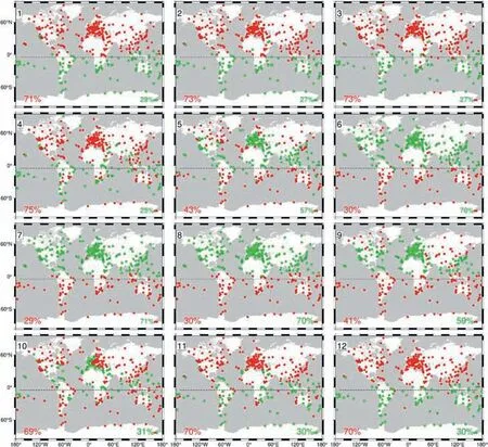
Fig.9. Monthly(January-December positive(green)and negative(red)categorization of the mean values for the differences between the predicted and the real ZWD values for all the 505 stations of the testing data (2017-2019).

Fig.10. 6-h time resolution 00:00(1),06:00(2),12:00(3)and 18:00(4)UTC Positive(green)and negative(red)categorization of the mean values between the predicted and real ZWD values for all the 505 stations of the testing data (2017-2019).

Fig.11. Mean values for the differences between predicted and real ZWD for 3 years testing data relative to the height (a) and latitude (b) of the station.

5. Conclusion

The Zenith Wet Delay (ZWD) is a critical component of GNSS meteorology and weather forecasting. In this research, ANFIS is implemented and suggested for the ZWD prediction. The ANFIS algorithm for forecasting the ZWD value over the next 6 h was tested using a 6-h data series from 505 geographically and spatially distributed from 2008 to 2019.

Two statistical criteria were used to evaluate the approach,and R values have been found to be 0.9, 0.8-0.9 and less than 0.8 for 85%,13%and 2%of the stations,respectively.The stations with the highest and lowest latitude values have exhibited strong correlations between the predicted and real value of the ZWD. Although coastal stations have the lowest R values,the predicted and the real ZWD accuracy is better in inland locations, as evidenced by previous studies. The RMSE values were then utilized, and it was revealed that 8.91%of the total stations(505 stations)had equal or less than 1 cm accuracy while the majority of the remaining stations (76.44% of the total stations) have accuracy in the range of 2 cm.The most intriguing result of this analysis is that 501 stations of the 505 globally and spatially distributed stations(99.21%of the total stations),have RMSE values equal to or less than 3 cm for the 3 years of testing data with 6-h time resolution,with only 4 stations having RMSE greater(0.2 mm) than 3 cm.

These RMSE values are associated with the station height.As the station height increases,it is expected that the predicted ZWD will become more accurate.While the same stations with RMSE values more than 2.5 cm are in symmetrical latitude zones, given the enhanced accuracy compared to the latitude greater than 60and less than -60.

Although the mean values of the differences between the predicted and the real ZWD values may be low as 1 mm, which is ineffective for weather forecasts, while a seasonal correlation was found,suggesting the spatial variation of the mean values.The level of accuracy attained in this study would be critical for weather forecasts and GNSS meteorology.

Data availability

The original data used in this study are available from:(https://vmf.geo.tuwien.ac.at/trop_products/gnss/vmf3/vmf3_op/yearly/).In addition,the data for each of the 505 stations containing the date with its ZWD value based on 6-h time resolution and the results for each station are available through https://10.17632/mcwnx2fypx.1.

Authorship statement

Conception and design of study

: Jareer Mohamm

ed;

tion of data:Jareer Mohammed;analysis and/or inte

rpretation of

data: Jareer Mohammed; Drafting the manuscript: Jareer Mohammed; revising the manuscript critically for important intellectual content:Jareer Mohammed.Approval of the version of the manuscript to be published: Jareer Mohammed.

Con

fl

icts of interest

The authors declare that there is no conflicts of interest.

Acknowledgments

This research did not receive any specific grant from funding agencies in the public, commercial, or not-for-profit sectors.