Data-driven parity-time-symmetric vector rogue wave solutions of multi-component nonlinear Schr¨odinger equation

Li-Jun Chang(常莉君), Yi-Fan Mo(莫一凡), Li-Ming Ling(凌黎明), and De-Lu Zeng(曾德炉)

School of Mathematics,South China University of Technology,Guangzhou 510640,China

Keywords: nonlinear Schr¨odinger equation,vector rogue waves,deep learning,numerical simulations

1. Introduction

Nonlinear Schr¨odinger(NLS)equations generally can be used to describe the nonlinear wave phenomena in diverse physics fields and have attracted more and more attention especially in hydrodynamics, nonlinear optical fibers, planar wave guides, and Bose–Einstein condensates theory.[1–5]For the integrable NLS systems,there exist lots of exact solutions including solitons, breathers, and rogue waves (RWs). They are all nonlinear waves with localized structure both in time and space. Note that, on the one hand, some solitons will produce breathers when they are disturbed periodically. And the RWs are the limit form of the breathers. On the other hand, solitons are stable waves and invariant of shape in the evolution under vanishing background, while RWs are unstable waves and the variation of shape in the evolution under non-vanishing background due to modulation instability. Especially,the amplitudes of RWs are usually two times or even higher than those of its surrounding waves, hence they frequently cause sea accidents and pose a great threat to people’s navigation safety for years. RWs were firstly constructed analytically by Peregrine,[4]expressed by the first-order functions.But these solutions did not get much attention until Solliet al.observed optical RWs in an optical fiber experiment.[6]Zakharovet al.[7]found the physical mechanism of usual RW generation was frequently related with modulation instability.Afterwards, RWs of different physical systems were one after another derived by related Darboux transformation.[8–16]Furthermore, recent studies have shown that the vector RWs ofn-component NLS equations are thePTsymmetry under the constraints of some parameters and classified intontypes in terms of the degree of polynomials.[17–19]In this paper, our research concentrates on data-drivenPT-symmetric vector RW solutions for the focusing multi-component NLS equation with nonzero boundary conditions:

In the last decades,deep learning has achieved great success in a wide variety of areas because of strong data representation ability, such as image processing, speech recognition, natural language processing, and many more.[20–24]Since neural networks (NNs) are universal approximation of functions,[25]as we know, it is natural to solve differential equations using NNs. Lagariset al.[26]presented a method to solve ordinary differential equations(ODEs)and partial differential equations(PDEs)by artificial neural networks(ANNs)for a given form of trainable solution. Sirignsnoet al.[27]introduced deep Galerkin method (DGM) to solve high dimensional PDE by Monte Carlo method for fast computation of second derivatives and an integral along its respective domain under proper measurement. Raissiet al.[28]put forward physics-informed neural networks (PINNs) method to solve PDEs and inverse problems through automatic differentiation technique(AD)[29]by random sampling points in the space domain. After that the variations of PINNs[30–46]have widely applied to solve distinct kinds of PDEs over years. Linet al.[35]utilized the two-stage PINN to simulate abundant localized wave solutions of integrable equations by introducing the measurement of conserved quantities into mean squared error loss method. Puet al.[36–38]proposed the improved PINN with neuron-wise locally adaptive activation function to simulate vector localized waves of Manakov system such as one-rational soliton solutions, RWs solution,breathers,and their interaction solutions. Wanget al.[39]combined the classical spectral method with PINN algorithm to correct the error perturbation caused by modulation instability on boundary problem and further simulate more accurate RW or breather solutions of NLS equation with a smaller numerical error for long time. However,mainly due to the difficulties of the computational complexity and the algorithmic instability in solvingn-component coupled nonlinear equations,previous studies of data-driven RWs mostly focused on one-component systems. The dynamical behaviors and relevant patterns of data-driven RWs of multi-component systems such as two- and three-component are less studied with deep learning method. Recently, in this respect, Moet al.[42]proposed the MS-PINN algorithm which picks the pre-fixed points for training the network again to simulate the datadriven degenerate/non-degenerate vector solitons for coupled NLS equation with the zero boundary theory. The MS-PINN algorithm combines the multiple thoughts of time-adaptive,adaptive sampling of collocation points, error measurement,and adaptive-weight[34,43–45]and obtains good numerical results on 2-NLS systems in the rectangle shape domain. Penget al.[46]used the Riemann–Hilbert method and PINN algorithm to solveN-double poles solutions for the non-local Hirota equation with nonzero boundary conditions. Inspired by above some papers,one of our goals of this work is to extend the zero boundary theory to the non-zero ones for the vector NLS equation with the MS-PINN algorithm.[42]In addition,we use the elliptic andX-shape spatio-temporal boundary conditions to simulate thePTsymmetric RWs of 2-NLS and 3-NLS systems.To the best of our knowledge,these results have never been reported before.

The structure of this paper is assigned as follows. In Section 2, we introduce briefly the PINN algorithm and give detailed descriptions about MS-PINN training method. In Section 3, we use the MS-PINN to simulate data-driven vector RW solutions of the 2-NLS system(1)in elliptic and X-shapes domains. Meanwhile, data-drivenPT-symmetric two-vector RW solutions of the 3-NLS system are also studied. In Section 4,some conclusions and discussions are given.

2. Multi-stage physics informed neural networks

In general,if we want to solve Eq.(1)by using deep learning,the most common neural networks are PINNs.The PINNs set up a deep neural network with the inputx,t,and the outputq(x,t), such that the output values can well approximate the solution of Eq. (1). PINNs take physical informationf(x,t)defined by Eq.(2)into consideration and use it as a part of the total loss functions on the spatio-temporal domain beside satisfying the initial and boundary conditions.And then we minimize the loss function through the optimization algorithm such as Adam[47]or L-BFGS[48]in order to obtain the optimal parameters. Define the residual functionf(x,t)ofn-component NLS system Eq.(1)below

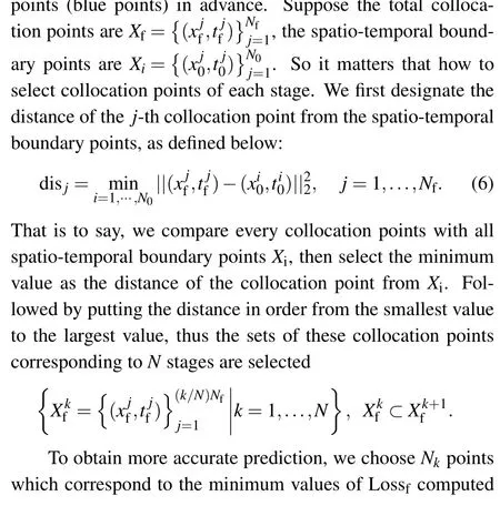
In the multi-stage physics informed neural network(MSPINN) algorithm, as shown in Fig. 1, we do not sample data points in the boundary region and the initial region respectively according to the traditional classical sampling method, but choose the adaptive spatio-temporal boundary points in manner of surrounding sampling on time and space together. Take the elliptic domain as an example,as displayed in Fig. 1(a), we first treat the boundary points of the elliptic domain in the direction of time and space as the spatiotemporal boundary points(yellow point)and then decompose the whole domain intoNparts which are kept apart from the spatio-temporal boundary points, forming one-to-one correspondence stages. Each stage we collect some collocation

Fig.1. Adaptive sampling collocation points in space-time. (a)and(b)The pre-fixed points from the one stage next stage the in elliptic domain and X shape domain,respectively.

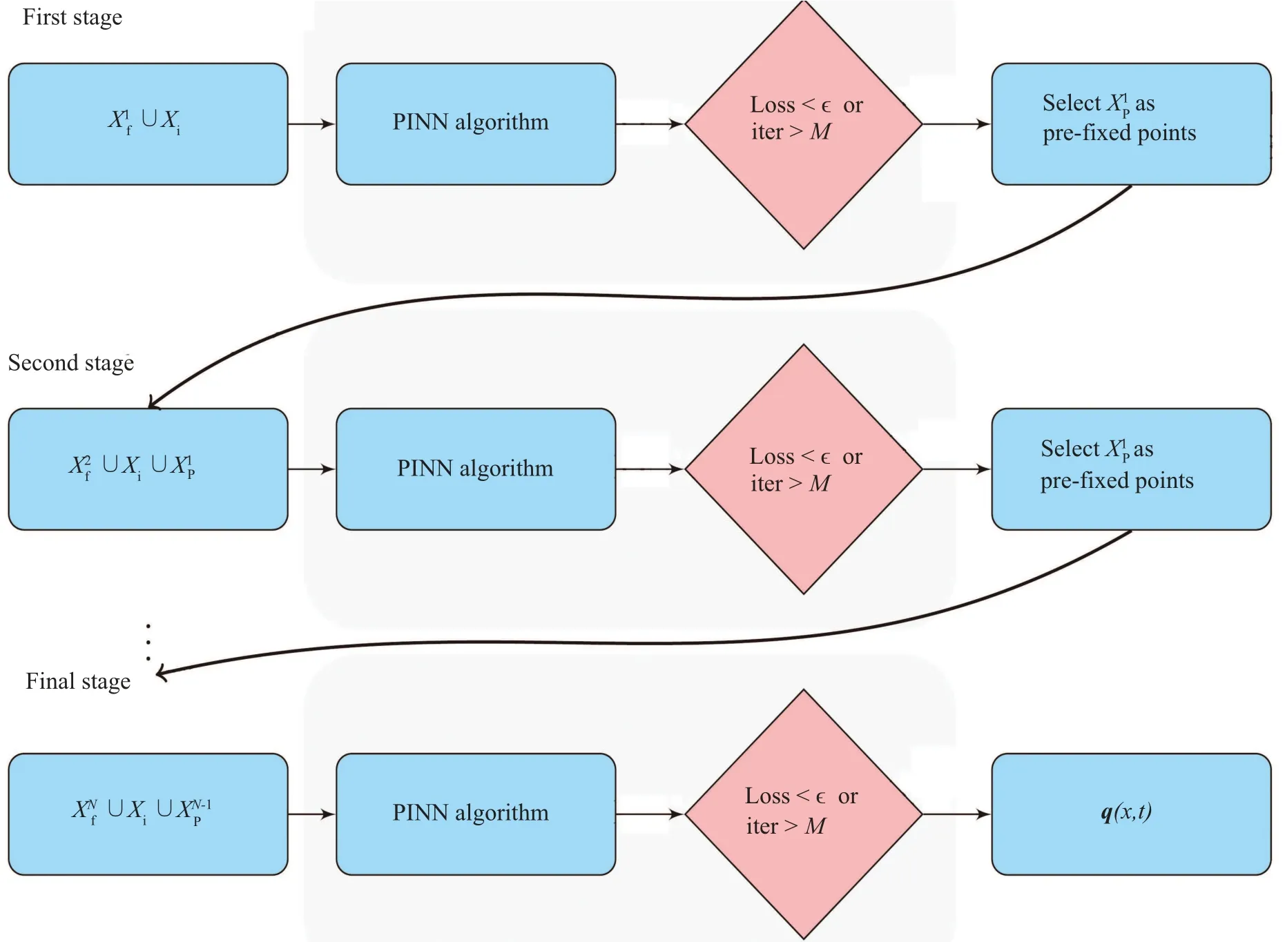
Fig.2. The MS-PINNs architecture. The first stage: the input X1f ∪Xi. By PINN algorithm the pre-fixed points X1P are obtained. The second stage: the input are X2f ∪Xi ∪X1P. By PINN algorithm,we obtain pre-fixed points X2P. The last stage: the input is XNf ∪Xi ∪XN-1P . By PINN algorithm,the output is q(x,t).

To more clearly represent the algorithm flowing-chart,we give the model architecture, as shown in Fig. 2. In the 1-st stage the inputs are the collocation pointsX1fand spatiotemporal boundary pointsXi, then we train the parameters by using PINN algorithm. When the loss function less than the given threshold value or the training iteration reaches our setM,we manually select theX1Ppre-fixed points which contribute to the smallest loss value of Lossf. Similarly,in the 2-nd stage the inputs areX2f,Xi,andX1P,we still train the model using PINN algorithm and when the loss function less than

3. Data-driven PT symmetric rogue waves of n-NLS equation

RWs,as a special type of nonlinear waves,have attracted more and more attentions in optical systems and other scientific disciplines. Recently, many studies onPT-symmetric vector RW solutions in anyn-component NLS models have also been proposed. However, due to modulation instability mechanism and the difficulty of observational conditions for RWs, we do not have a complete understanding of RW phenomena. Thus in this section,we would like to precisely simulate thePTsymmetric vector RW solutions of 2-NLS and 3-NLS systems with the non-zero spatio-temporal boundary conditions by MS-PINN algorithm.

3.1. The PT symmetric fundamental vector RW solution of 2-NLS system

Specifically,the fundamental vector RW solutions forj=1,...,n,where

aj=ζcscωj,bj=ζcotωj,aj,bj,α0,ζ,ωj ∈R are the parameters which nontrivially contribute to the profile of the vector RWs. ThePT-symmetric structure of a vector RW isqj(x,t)=PT qj(x,t)=Pq*j(x,-t).Tis the conventional bosonic the time-reversal operator:t →-t, i→-i, where*denotes the complex conjugation.

For a 2-NLS system, we can obtain explicitly the vector RW solutionq(x,t)=(q1(x,t),q2(x,t)) with the parametersω1=π/3,ω2=2π/3,ζ=1,α0=-1/2,t ∈[-1,1],x ∈[-4,4]by Eq.(9).We simulate the data-driven vector RWs by deep neural network with 3 hidden layers and 50 neurons per hidden layer.The activation function is the hyperbolic tangent (tanh) function. By dividing the whole domain into 4 parts and following 4 stages,we set the numbers of total collocation pointsNf=2×104,spatio-temporal boundary pointsN0=200 and pre-fixed pointsNk=(0.6k/4)Nf=3×103k,(k=1,...,4) which means 60% of collocation points are selected as pre-fixed points. In each stage the number of iterations of is 5000 and the learning rateεis 1e-4 for training with optimizer L-BFGS.

We know RWs usually admit one peak and two valleys,one valley and two peaks and two peaks and two valleys. For the RW of scalar NLS equation,RW usually has one peak and two valleys and the maximum amplitude is twice height of the background field. For the RWs of multi-component NLS equation,there exist the bright,dark and four-petal type RWs,which are the generalization of classic RWs. For more information about the classification of fundamental RW types,please refer to these articles.[18,50,51]Each componentqjof the 2-NLS system is a kind of the fundamental RW and the types of the structures are controlled byωj. As shown in Fig.3,q1andq2are eye-shaped RWs with one hump and two valleys in top panel. Then we take relative L2(RL2)error as evaluation metrics in order to validate the method with simulated data.At the same time,considering the effect of noise in real-world observations, we add 5%white noise data and 10%white noise data to the spatio-temporal boundary condition. As shown in Fig.4, the absolute error|q1|+|q2|of the MS-PINN method is nearly 30 times less than that of the PINN method. The absolute errors of the MS-PINN method with 5%and 10%white noise data still nearly 20 times and 6 times less than PINN algorithm.

Fig.3. The intensity of PT symmetric vector RW solutions of the 2-NLS system simulated by the MS-PINN algorithm in elliptic area and the comparison between the intensity of the predicted solutions and accurate solutions of two components system at times t =-0.5 and t =0 corresponding to the two temporal snapshots depicted by the blue vertical lines in the top panel.

Fig.4. The absolute error|q1|+|q2|of PINN method,MS-PINN algorithm with clean data,MS-PINN algorithm with 5%white noise data and with 10%white noise data.

Fig. 5. The intensity of PT symmetric vector RWs of the 2-NLS equation simulated by the MS-PINN method in X-shape domain and the comparison between the intensity of the predicted solutions and accurate solutions of two components system at times t =-0.5 and t =0 corresponding to the two temporal snapshots depicted by the blue vertical lines in the top panel.

In order to explain the applicability of the algorithm in complex geometry domain for 2-NLS equation,we replace the oval region with the X-shape domain,as shown in Fig.5. By the comparison between the predicted solutions and exact solutions of 2-NLS equation,we find the MS-PINN algorithm also well approximate the exact solution. Figure 6 shows the absolute error of the PINN method is about much 100 times,30 times,and 10 times larger than those of the MS-PINN method with clean training data, 5% white noise data and 10% white noise data, respectively. It can be seen that the data-driven solutions of nonlinear coupled system can be still kept relatively stable against the small perturbation.

Fig.6. The absolute error|q1|+|q2|of PINN method,MS-PINN algorithm with clean data,MS-PINN algorithm with 5%white noise data and with 10%white noise data.

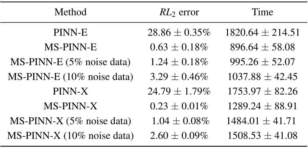
Table 1. The comparison of the PINN method and MS-PINN method base on 5 independent repeated experiments for 2-NLSE in elliptic-and X-shape regions.

Because the neural network may get different solutions from different initial data, we train the neural network from random initialization for 5 times. More detailed information aboutRL2error and time cost with PINN method and MS-PINN algorithm in elliptic-and X-shape domains are displayed in Table 1. “-E,-X”denote the abbreviations of ellipse and X shape. PINN-E and MS-PINN-X represent the uses of the PINN and MS-PINN algorithm in ellipse and X-shape region,respectively.

3.2. The PT symmetric vector two-RW solutions of 3-NLS system

In the above subsection,we have simulated thePTsymmetric fundamental vector RW solutions of the relative 2-NLS equations and analyzed theRL2error of MS-PINN algorithm with 5%white noise data and 10%white noise data.To our knowledge, simulating asymptotic behaviors of thePTsymmetric vector RW solutions of 3-NLS system with deep learning has not been evaluated at present. For 3-NLS equation, we choose an exact vector two-RW solutionsq(x,t)=(q1(x,t),q2(x,t),q3(x,t))given by setting the special parameters[18]

We simulate the data-drivenPT-symmetric vector RW solutions by deep neural networks with 3 hidden layers neural network and 200 neurons per hidden layer. By dividing the whole domain into 4 parts, we have naturally 4 stages. The datadriven vector RW solutions of system resulted from the MS-PINN algorithm with the randomly chosen spatio-temporal boundary pointsN0=400,total number of collocation pointsNf=4×104and the number of pre-fixed pointsNk=(0.6k/4)Nf=6×103k,(k=1,2,3,4). In other words, we consider 60% of collocation points as pre-fixed points in trained domain for each stage. In each stage the maximum iterationMis 2×104and the learning rate thresholdεis 10-3with optimizer L-BFGS.

Figure 7 shows the intensity plots of 3-NLS equation onx ∈[-20,20],t ∈[-0.5,0.5].Top panel shows the density evolutions of 3-NLS system. Bottom panel shows the intensity of three components att=-0.25 andt= 0.25 corresponding to the two temporal snapshots depicted by the white horizontal lines in the top panel. Based on the classification of fundamental RW types,[18]the density plots ofq1andq3for the 3-NLS system are both four-petaled RWs sinceω1,ω3∈(π/6,π/3)∪(2π/3,5π/6),while the intensity plot ofq2is the bright RW due toω2∈[π/3,2π/3]. The simulation shows that the data-driven predicted solutions are very close to the exact solutions given before,which further demonstrates the observability of RWs in the physical experiments.

Fig.7. The intensity plots of the PT symmetric vector RW solutions of 3-NLS system simulated by MS-PINN method and the six plots of the comparison between the of the predicted solutions and accurate solutions of three components system at times t=-0.25 and t=0.25.

Fig.8. The absolute error|q1|+|q2|+|q3|of PINN method,MS-PINN algorithm with clean data,MS-PINN algorithm with 5%white noise data and with 10%white noise data,respectively.

The absolute error|q1|+|q2|+|q3| of the PINN method and that of the MS-PINN method (with clean data, 5% white noise data and 10% white noise data) are displayed in Fig. 8. Obviously, the MS-PINN method obtains much 50 times better experimental effect than that of the PINN algorithm on 3-NLS equation.Though we add some white noise data to spatio-temporal boundary condition, the absolute errors are still much less than that of the PINN algorithm. For 3-NLS system, more specificRL2errors and time costs with PINN method and MS-PINN algorithm with white noise data are shown in Table 2.

Table 2.The comparison of the PINN method and MS-PINN method base on 5 independent repeated experiments for 3-NLSE.

4. Conclusion

In this work,we utilize a multi-stage deep learning training algorithm to simulate data-drivenPT-symmetric vector RW solutions of 2-NLS systems and two-vector RWs of 3-NLS systems with spatio-temporal boundary condition (nonzero boundary condition). In fact, the spatio-temporal conditions do not conform to the traditional numerical methods of solving the equation in manner of time evolution,but comply with physics dynamics in the way of simultaneous evolution of time and space. Numerical simulations show that the MSPINN algorithm can well recover different dynamical behaviors of RW solutions in the 2-NLS and 3-NLS equations. In the future, we would like to explore whether the MS-PINN algorithm is applied to the discovery problems of other integrable NLS and non-integrable nonlinear wave system by adding more prior knowledge about the geometry and physical properties of system.

Acknowledgments

Project supported by National Natural Science Foundation of China (Grant Nos. 11771151, 61571005, and 61901160), the Science and Technology Program of Guangzhou (Grant No. 201904010362), and the Fundamental Research Program of Guangdong Province, China (Grant No.2020B1515310023).