Advantage of populous countries in the trends of innovation efficiency

Dan-Dan Hu(胡淡淡) Xue-Jin Fang(方学进) and Xiao-Pu Han(韩筱璞)

1Alibaba Research Center for Complexity Sciences,Hangzhou Normal University,Hangzhou 311121,China

2Institute of Information Economy and Alibaba Business School,Hangzhou Normal University,Hangzhou 311121,China

Keywords: innovation efficiency,population size,the relative indexes

1. Introduction

Over a long time in the past, technological progress was assumed to be an exogenous variable and independently determined the equilibrium level of economic development.After Romer and Lucas’ pioneering work of the endogenous growth model,[1,2]some economists revealed technology evolves endogenously,[3]and were gradually exploring how to germinate, accelerate, and improve technological change efficiently in this new complicated situation.[4–6]A substantial amount of relevant studies have thus consecutively emerged,in which a crucial focus is how the population relates to technological development.

As early as the last century,some researchers have found that a large population probably boosts innovation. They proposed as the population rises, so does the rate of technological progress.[7,8]Major innovation cycles must be generated at a continually accelerating rate to sustain growth and avoid stagnation or collapse.[9]In the paradigm of Boserup,population determines the pace of technological change,contributing to escaping the Malthusian trap.[10]Galor and Weil constructed a model which completely agrees with Boserup’s viewpoint and further suggests population size is the crucial factor that allows a transition from Malthusian to the post-Malthusian regime.[11]Additionally, Kremer combined a Malthusian equation with a technological change equation,building a highly stylized model where the technology growth rate is linearly proportional to the population,and to the population growth rate.[12]

Why is technological progress heavily dependent on population size? Some explanations are offered in Romer’s wellknown paper published in 1990.[8]Firstly,a large-scale group,equivalent to a large and diverse talent pool,can enable more people to engage in research and innovation, thereby driving faster technological progress and higher productivity. Gomez-Lievanoet al. revealed that the number of people engaged in ten different urban phenomena,including innovative activities,scales as a power law with population size.[13]Recently,Liang made it clear in his latest work that a large population seems to be the most important source of advantage for innovative activities and specifically summed up three channels of population size exerts on innovation.[14]Some recent studies also reported the impact of urban population size on urban innovation activity[15,16]and found the critical population of innovative cities.[17]Much historical evidence has proved that cities are the principal engines of innovation.[18]In Bettencourt’s canonical works,he suggested that most urban socioeconomic indicators fit power-law functions of population size with similar scaling exponents.[9,19]Later, Panet al. demonstrated that social-tie density scales super-linearly with population density in cities.[20]Loboet al. empirically found that there is a systematic dependence of urban productivity on city population size.[21]More empirical observations and theoretical explanations of scaling laws of urban population with urban metrics could be found in Gao’s review paper.[22]Furthermore, Liet al.mentioned that a local active population plays a deterministic role in the evolution of city populations, road networks, and socioeconomic interactions.[23]These findings provide implicit evidence for a positive correlation between population size and innovation.

More importantly, a larger population not only increases the supply of potential researchers but also stimulates demand for their services by expanding the size of the market.[24]Although the population is not an exact metric of market size,the population growth of a region is always in direct proportion to the size of its market.[25]Therefore,it is reasonable to treat a populous country as an extensive local market.

As for the significant and robust effects of market size on innovation, scholars in relevant fields have reached a consensus.[26,27]In the empirical study of the Chinese manufacturing industry, Beerliet al.found an increase in market size by 1 percent leads to an increase in firm-specific total factor productivity by 0.46 percent.[28]Total factor productivity is attributed to the evolution of technology by the famous economist Solow.[29]In Romer’s model,larger markets induce more research and faster economic growth. Gao and Jefferson argued that it is because large and fast-growing markets create a premium for research-intensive industries,[30]while Desmet deemed it due to more fierce competition.[31]In the study of the first industrial revolution,Deane pointed out that,it is only when the potential market is large enough, and demand elastic enough,to justify a substantial increase in output,that entrepreneurs break away from traditional techniques and turn to the door of new technology.[32]Indeed,only immense markets can bear the fixed costs of capital investment, and help entrepreneurs get profits from the adoption of new technologies.

Taken together, population size certainly relates to innovation. However, previous results were almost derived from theoretical research, few studies have attempted to prove the relationship between population size and innovation based on empirical analysis.In our study,we take innovation efficiency,the main driving force for prospective economic growth due to the scarcity of innovation resources,[33]as a metric of innovation performance in conducting our empirical research.

Innovation efficiency can be defined as the ratio of output over input, representing the ability of economies to translate innovation inputs into innovation outputs.[34]It is related to the concept of productivity. Innovation efficiency is improved when with the same amount of innovation inputs more innovation outputs are generated or when few innovation inputs are needed for the same amount of innovation outputs. Given the multi-input and multi-output of innovation systems, the data envelopment analysis (DEA) is widely applied to measure innovation efficiency. The DEA model has become relatively flawless through continuous modification and optimization. However, it dismays us that almost all studies use the raw data of innovation input and output,such as R&D investment, the number of patent applications and papers, neglecting the impact from the difference of economic development level.[35–37]In fact, innovative activity is closely linked with economic performance.[38]There are considerable technology differentials within innovation systems due to the differences in countries’economic development.[39]If we are reckless of this issue, corresponding to assuming that economies use the same technology to transform innovation inputs to innovation outputs,the cross-country comparison of innovation efficiency would not be accurate.[38]Because innovation efficiency itself is a reflection of the national technology level,it is unfair to compare economically developed and technologically advanced countries, such as the United States, with backward and developing countries.

In this paper, we propose three “relative indicators” by excluding the impact from the difference of economic development level,to accurately measure the innovation efficiency of each economy, and achieve the cross-country comparison.We reveal that all of the three relative indicators show significant correlations with population size,and discover the critical population. This present paper finds empirical support for the claim that population size is positively correlated with innovation efficiency. In the following sections,we firstly introduce the data sources and the construction of three relative indexes(Section 2), and then dig out the difference hidden in the trajectories of economies in several indicator spaces(Section 3),as well as the correlation between the trends of innovation efficiency and population size of economies(Section 4),finally conclude our study together with a discussion of limitations and further research(Section 5). As we will introduce below,we find that the economies with a larger population size have better performance on the trends of innovation efficiency.

2. Data and methods

2.1. The datasets

The datasets used in our analysis are all derived from the database of the World Bank(https://www.worldbank.org/),including the number of patent applications, Research and Development (R&D) investment, the gross domestic product(GDP), population and income per capita of each economy over the period from 1985 to 2019. The details of two major datasets can be found as follows:

(i)The number of patent applications

Patent applications of each economy are granted through the Patent Cooperation Treaty procedure or its national patent office. It is one of the major types of outputs on innovation.The data of 153 economies all over the world is collected.(ii)The R&D investment

The R&D investment refers to both current and capital expenditures of systematic innovation efforts,usually representing the level of innovation input.[40,41]In our study,R&D investment is calculated using R&D investment as a proportion of GDP and GDP. After removing the null and the double-counted,we retain 149 economies including all major economies and large population centers.

2.2. The relative R&D cost per patent

Generally, the innovation efficiency of an economy can be measured by the cost of innovation and the outputs of innovation,respectively.The lower the cost,the higher the outputs,the higher innovation efficiency. A natural metric of the cost of innovation is the investments required to produce a patent application. Therefore R&D cost per patent, which refers to R&D investments required for each patent application,is used to be the basic indicator of innovation efficiency. R&D cost per patent is defined as

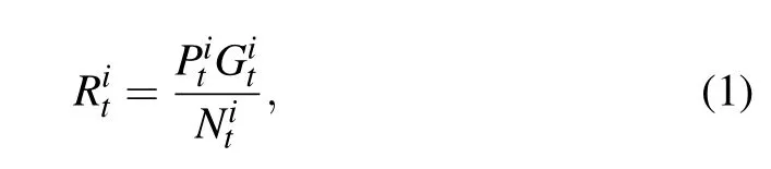
whereRitis R&D cost per patent, representing the average R&D cost required for each patent application of economyiin yeart, andPit,Git, andNitare R&D investments (as a proportion of GDP),GDP,and the number of patent applications of economyiin yeart,respectively. It should be noticed that R&D cost per patentRis not an exact average cost for each patent application,since R&D investments are not all invested in patent development and the patent application is not all of the R&D outputs. Indeed,it is hard to get the exact investment on patent development of each economy,butRcan reflect the level of cost on patent development in cross-country comparison to a large extent because the patent is the representative part of R&D output and the number of patent applications also is widely used as an effective key indicator of R&D output.

However, as mentioned above, the great disparity on the development level between different economies would strongly impact the level of R&D cost per patent and weaken the effectiveness of the direct comparison using R&D cost per patent,since economies at different stages of development may have different modes of innovation system. The impact of economic development level thus should be eliminated before the comparison on R&D cost per patent. The method is introduced as follows:

Firstly,we plot the trajectory of each economy in a space of GDP per capita and R&D cost per patent. For GDP per capita,because the value of GDP per capita is impacted by the exchange-rate shift,we use standard GDP per capita instead of it. The standard GDP per capita is defined as the ratio between the GDP per capita of an economy in a year and the global average of GDP per capita in the same year. Since the strong heterogeneity in the distribution of GDP per capita, the logarithmic value of the standard GDP per capita is used in this analysis:

After taking a logarithmic of the original values,the data points in different years generally distribute in the same range,indicating that the data of each economy in different years have been efficiently incorporated into a standardized space(gandr). As shown in Fig. 1(a), we get the trajectories of economies in the space. Note that China and India’s trajectories are strikingly different from others due to their downward trend. It means the R&D cost per patent in both economies decreases as the economy grows. Averagely speaking,ris positively dependent ong.

We process all the data points in the space as a whole and use the moving average method to obtain the mean curve(the dashed curve in Fig.1(a)). The width of the moving window in this calculation is fixed as 0.5 to balance the accuracy ongand the data size in the moving window. This mean curve represents the global average ofrfor the economies with similar economic development levels, points out a natural trend ofrdepending on the economic development at the global level, and gives us a set of benchmarks to judge how much an economy’s R&D cost per patent is higher or lower than the case with natural growth. For an economy with the R&D cost per patent just on the global expectation level, its trajectory in this space should follow the mean curve in its economic development. The data point above the mean curve indicates that the R&D cost per patent of the corresponding economy already exceeds the level of global expectation at the current economic level, that is to say, the economy’s innovation process is not efficient enough. The higher the data point leaves the mean curve, the higher the R&D cost per patent, signifying the weaker the economy’s efficiency on the transformation from innovation input to innovation output, even though the absolute level on the innovation output possibly is high(for some high-income economies). The one below the mean curve means the opposite case. It inspires us that, the deviation of each economy’s data point from the mean curve can be used as a new benchmark to evaluate an economy’s real level on R&D cost.

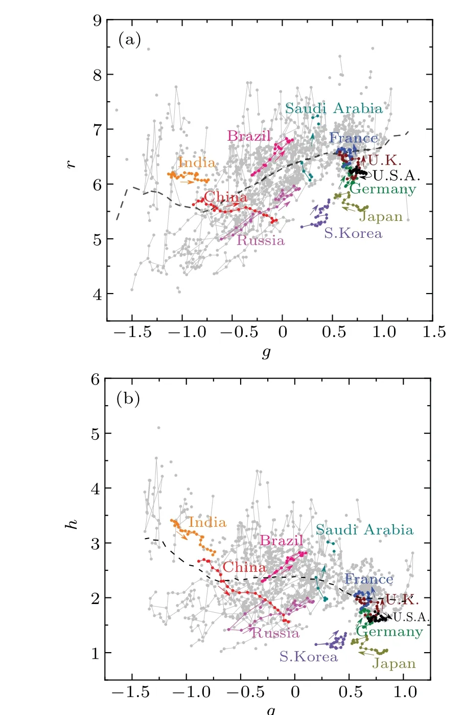
Fig.1.The trajectories of economies in the space of the logarithmic standard GDP per capita(g)and the logarithmic standard value of two types of cost per patent: (a)the logarithmic standard value r of R&D cost per patent from 1996 to 2018,(b)the logarithmic standard value h of holistic labor cost per patent from 1996 to 2018. The colored curves correspond to the trajectories of 11 representative economies, and the gray curves show the trajectories of other economies. The colored arrows depict the direction in which the trajectories move. The dashed line in each panel is the mean curve created by the moving window with a width of 0.5.

Previous studies have found that this type of relative index shows better performance on the metric of innovation capability.[42]Similarly, since almost all the indicators relevant to innovation efficiency are strongly impacted by the economic development level, they are also converted to be their relative indexes in our analysis.

2.3. The relative holistic labor cost per patent

The R&D cost per patent can partially reflect the level of the cost of innovation. However, because of the large differences in the labor costs in different economies,the R&D cost per patent can not directly reflect how much workload can support a patent application in the economy. We thus propose a metric called “the holistic labor cost” to measure the level of this workload. The holistic labor costHis defined as the ratio of the R&D cost per patent to income per capita:

whereHitis the holistic labor cost required for each patent of economyiin yeart,Ritis the R&D cost required for each patent of economyiin yeart,andEitrepresents the income per capita of economyiin yeart. Obviously,His a type of time length and represents the labor cost on time that can support a patent application in the economy.In other words,His not the average labor investment on a patent application but a holistic labor cost on time at the level of the economy.

Similarly, we replace the original value with the relative holistic labor cost per patent, which is constructed in exactly the same way as the relative R&D cost per patent. It can be simply summarized as follows: We first plot the trajectory of each economy on a space ofhandg, wherehis the logarithmic standard value ofH, as shown in Fig. 1(b), and then get the mean curve through a moving window with a fixed width of 0.5, and calculate and standardize the deviation from each data points to the mean curve, finally the standardized deviationIhis the relative index of the holistic labor cost per patent.

2.4. The relative index of innovation output

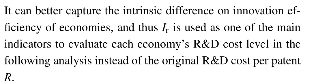
Besides the above two relative indexesIrandIhmeasuring the level of innovation cost,we also analyze the innovation efficiency of economies by measuring the level of innovation output. The natural metric of innovation output level is the number of patent applications per capitan, which is mightily dependent on both the economic development level and the innovation input level.The innovation input level of an economy can be reflected by the percentage of the R&D investments in GDPp, also depending on the economic development level.We thus first build the relative index of the number of patent applications per capita and the relative index of the percentage of the R&D investments in GDP,to exclude the impact of economic development level. The construction method of the two relative indexes is exactly the same as that ofIrandIh,in which the original indicatorsRandHare just respectively replaced asnandp, as shown in panels(a)and(b)of Fig.2.Using this method,two relative indexesInandIpare obtained,corresponding tonandprespectively.

The trajectory of each economy in the space of the two relative indexesInandIpare shown in Fig. 2(c), and showing an obvious correlation betweenInandIp. Its reason is that the innovation outputs also depend on the innovation input level.We further eliminate the impact ofIpfromIn,and the standardized deviation from each data point to the mean curve(getting using the moving window with width 0.5)is used to be a new relative indexIo, which expresses an expected level of innovation output(patent applications)of the economy in the condition assuming all economies have the same economic development level and the same innovation input level.Iois the relative index of innovation output that will be used in the following analysis.

Fig. 2. (a) The trajectories of economies in the space of the logarithmic standard GDP per capita g and the logarithmic standard number n of patents per capita. (b)The trajectories of economies in the space of g and the logarithmic standard percentage p of the R&D investments in GDP.(c)The trajectories of economies in the space of the relative percentage of the R&D investments in GDP and the relative number of patents per capita. The colored curves correspond to the trajectories of 11 representative economies, and the gray curves show the trajectories of other economies. The colored arrows depict the direction in which the trajectories move. The dashed line in each panel is the mean curve created by the moving window with a width of 0.5.

3. Trajectory analysis

An obvious feature presented in Fig.1 is that with the economic development, economies with large populations (such as China and India)have a glaringly downward trend in both the R&D cost per patent and the comprehensive labor cost per patent. What is more,as can be seen from Fig.2(c),the relative number of patents per capita of economies with large populations is constantly improving over the period from 1996 to 2018, especially the curve of China. In view of these phenomenons, it is reasonable to suspect that the trends of innovation efficiency would be correlated to population size.

To test our conjecture, we first analyze the trajectory directions of economies with different populations,which present the apparent discrepancy in Figs. 1 and 2.All economies are divided into three groups according to population＜2×107(Group 1), 2×107＜population＜2×108(Group 2) and population＞2×108(Group 3). Given the characteristics of population growth, “population”here is the geometric average of the population from 1996 to 2018 for each economy. Before the comparison,standardized treatment is needed to put the trajectories in different indicator spaces into a same comparable square framework. Taking the Fig.1(a)for an example,gandrare replaced by Δg′and Δr′:

Exactly the same way is used to compute the azimuth angle of trajectories in Figs. 1(b) and 2(c). To balance the data size,the sliding window is fixed as 10°to count the frequency from-180°to 180°. The normalized frequency distributions of the azimuth angle are shown in Fig.3,in which panels(a),(b), and (c) show the azimuth angle distribution of the R&D cost per patent,the holistic labor cost per patent and the index of innovation output,respectively.In each panel,the blue area,the green area and the red area represent Group 1,Group 2,and Group 3,respectively.

As shown in Fig.3,there are apparent differences among the three groups,especially between Group 3(the group with the largest population size)and the other two groups.In panels(a)and(b),the most probable value of the coordinate azimuth angle of each group decreases as the typical population size of the group increases. The coordinate azimuth angle of Group 1 and Group 2 are mostly concentrated on the range(30°,90°),which means the R&D cost per patent and the holistic labor cost per patent is going along with the growing economy.Conversely,the coordinate azimuth angle of Group 3 is strikingly negative (mainly in the range-90°and 0°), indicating that economies with population size more than 2×108typically cost less to invent a patent,both the R&D cost and the holistic labor cost.

Similarly, figure 3(c) also shows the obvious difference between Group 3 and the other two groups. Group 1 and Group 2 are mostly distributed in(-180°,0°)while Group 3 in(0°,180°),showing that the economies in Group 3 have more possible to show an improvement trend on the level of innovation output. All of the above results emphasize that the larger the population,the better the tendency of innovation cost and innovation output.

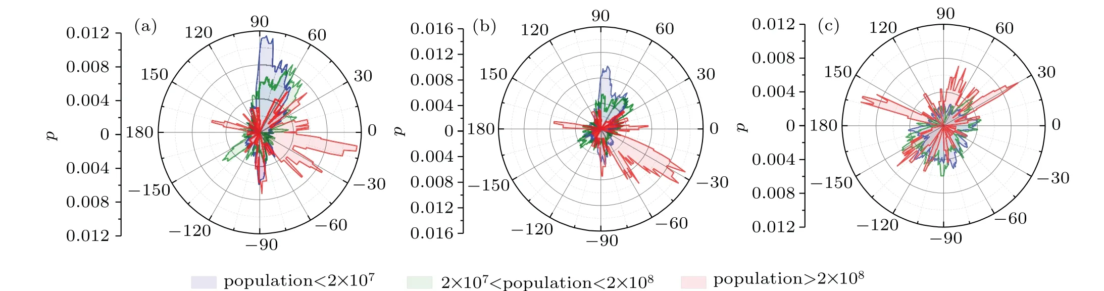
Fig.3.The distribution of coordinate azimuth angle of the trajectories in Figs.1(a),1(b)and 2(c).Panels(a),(b),and(c)respectively correspond to Figs.1(a),1(b),and 2(c). The blue,green,and red curves correspond to the groups of population ＜2×107,2×107 ＜population ＜2×108 and population ＞2×108,respectively.

4. Correlation analysis

To exactly investigate the relationship between the trends of innovation efficiency and population size of the economy,the change of three relative indicators(the relative R&D cost per patentIr, the relative holistic labor cost per patentIh, and the relative index of innovation outputIo) of each economy above over the period from 1996 to 2018 is calculated simply using the last year’s value minus the first year’s value. For example, the change ofIris ΔIr=Ir|2018-Ir|1996. For the economies with missing 1996 or 2018 data, we replace the missing data with the data of the nearest adjacent years in the period from 1996 to 2018.For instance,if an economy is missing data for 1996 and 1997, and thus its 1998 data is used as the first year’s value.Obviously,ΔIrand ΔIhare lower,and ΔIois higher,which means a better trend of innovation efficiency.

The scatterplots of the relationships between the changes(ΔIr,ΔIh,and ΔIo)and the population size of each economy are shown in Fig.4.Notice that,the value of the population size of each economy is the geometric average of the economy’s annual population in the period from 1996 to 2018 because the population size of each economy changes every year. For the economies with missing 1996 or 2018 data,the start year and the end year of the period of geometric average of the annual population are replaced by the nearest adjacent years in the period from 1996 to 2018. Also using the previous example,for an economy with missing data for 1996 and 1997, the period of its geometric average of the annual population is from 1998 to 2018. In Fig. 4, the total number of economies shown in panels(a),(b),and(c)is 109,97,and 109,respectively.Correspondingly,in the three panels,the total number of economies with no data missing is 41,37,and 41,respectively.

As the features plotted in Fig. 4, most economies have positive ΔIrand ΔIh, and negative ΔIo, implying that their innovation cost tends to increase and the efficiency of their innovation output tends to reduce. In other words, innovation efficiency in most economies does not show an improvement trend.

All the three relationships shown in Fig. 4 can be well linearly fitted,and the fitting slopes are-0.467,-0.513,and 0.442 respectively. Correlation analysis shows that ΔIr, ΔIh,and ΔIoare all significantly correlated with the population size with the significance levelP ＜5×10-4(the three panels in Fig.4). The correlations of ΔIr(Fig.4(a))and ΔIh(Fig.4(b))is negative, and the Pearson correlation coefficientsrrespectively are-0.37 and-0.38, indicating that the economies with large population size tend to have smaller increase on the innovation cost. The positive correlation between ΔIoand population size (the Pearson correlation coefficientr=0.34,as shown in Fig.4(c))shows that the efficiency of innovation outputs of the economies with large population size usually have smaller decline,which also indicates an advantage on the trends of innovation efficiency.

Fig.4. The correlations between the change of three relative indicators and the logarithm of population size: (a)The difference of the relative R&D cost per patent Ir between 1996 and 2018. (b)The difference of the relative holistic labor cost per patent Ih between 1996 and 2018. (c)The difference of the relative index of innovation output Io between 1996 and 2018. The colored data points correspond to the 11 representative economies, and the gray circles denote other economies. In each panel, the linear fitting result is shown by the dashed line, the dashed dot line shows y=0, and the x value of the cross point is denoted by the vertical dot line.

All fitting lines in Fig.4 have a cross point with the liney=0. Thexvalues (the logarithmic population size) of the cross points are 8.75 for ΔIr, 8.34 for ΔIh, and 8.97 for ΔIo,respectively, which correspond to the population size about 0.56 billion,0.22 billion,and 0.93 billion,respectively. From the left side to the right side of the cross point,the innovation efficiency transforms from a downward trend to an improvement trend in an average sense. The cross point, therefore,indicates the critical size of the population,revealing that averagely speaking,the economies with a huge population(over the critical size of population)have an endogenous advantage to produce positive feedback that can spontaneously improve their innovation efficiency.

We further observed that the stability of the trends of innovation efficiency is also correlated to the economy’s population size. For each economy,the standard deviations of the annual change(σ(ΔIr),σ(ΔIh),andσ(ΔIo))of the three relative indexes(Ir,Ih,andIo)are calculated respectively to represent the economy’s stability of the trends of innovation efficiency.The correlations between the population size and the standard deviations of the three relative indexes during 1996–2018 are shown in Fig.5. The standard deviations are all significantly negatively correlated with population size (The P-value are all smaller than 5×10-3),and the Pearson correlation coefficientsrrespectively are-0.50,-0.41,and-0.30,indicating that the economy with a larger population has a more stable trend in innovation efficiency.

Figure 5 also contains the information of the average of standard GDP per capitag(shown by the color of each data point) and the average annual growth rate ofg(denoted by the diameter of each data point) of each economy over the period 1996–2018. The economies with different economic development levels and different economic growth rates are clearly clustered in different regions of Fig.5. In every panel of Fig. 5, the high-income economies are mostly below the fitting lines, indicating the high-level stability on the change of innovation performance of these economies. The rapidly developing economies are mainly concentrated in the regions close to the fitting lines,implying the relative position of each economy’s data point may be related to the speed of economic growth.

Fig.5. The correlations of population size and the standard deviation of the annual change in the three relative indexes during 1996-2018. Logarithms are taken for both population size and the standard deviation. The relative index in panels (a), (b), and (c) respectively is Ir, Ih, and Io, and σ represents their standard deviations of the annual change in these relative indexes. The color of data points correspond to the average of the standard GDP per capita g over the period 1996–2018,and the diameter of each data point is proportional to the average annual growth rate of g from 1996 to 2018. The dashed line shows the linear fitting in each panel.

Fig. 6. The relationship between the average annual growth rate of standard GDP per capita 〈Δg〉 and the deviation of the standard deviation of the annual change in the three indexes δ[log10 σ(ΔI)] from 1996 to 2018. Panels (a), (b), and (c) respectively show 〈Δg〉 versus δ[log10 σ(ΔIr)], 〈Δg〉 versus δ[log10 σ(ΔIh)], and 〈Δg〉 versus δσ(ΔIo). The color of data points shows the average of g over the period 1996–2018. The dashed lines are given with Gauss function fitting, in which the peak points respectively are at δ[log10 σ(ΔIr)]=0.15 for panel (a), δ[log10 σ(ΔIh)]=0.15 for panel (b), and δ[log10 σ(ΔIo)]=0.21 for panel(c).

To analyze this relationship,for each panel of Fig.5,we calculate the vertical deviation between data points and the fitting line to represent the relative stability of economies’trend in innovation efficiency:

whereδ[log10σ(ΔI)] is the deviation ofσ(ΔI),σ(ΔI) is the standard deviation of the annual change in the three indexes,and〈log10σ(ΔI)〉is the corresponding level of log10σ(ΔI)on the fitting line. Note thatIrefers toIr,Ih,andIo,corresponding to panels(a),(b),and(c)of Fig.5,respectively. Actually,δ[log10σ(ΔI)]can be seen as the relative stability on the trend of innovation efficiency excluding the differences onσ(ΔI)caused by population size.

Figure 6 plots the relationship between the average annual growth rate ofgand the vertical deviationδ[log10σ(ΔI)](hereI=Ir,Ih,andIo).In all panels,the high-income economies are concentrated in the lower left of space. Overall, with the increase ofδ[log10σ(ΔI)],〈Δg〉rises and then decreases, presenting an obvious unimodal shape that can be roughly fitted by Guass function. The peaks of fitting curves respectively are atδ[log10σ(ΔIr)]=0.15,δ[log10σ(ΔIh)]=0.15,andδ[log10σ(ΔIo)]=0.21, possibly indicating an optimized stability level that balances the fluctuation on the growth of innovation performance and the economic development.

5. Conclusion and discussion

This paper proposes the three relative indicators to measure and compare the innovation efficiency of economies after excluding the impact of economic development level and observes the advantage of economies with large population sizes in the trends of innovation efficiency. A key method in this study is the construction and the adoption of the relative indexes for innovation efficiency. Different to analysis on the traditional innovation indexes,[39]these relative indexes exclude the impact of economic development level and put all economies into a comparable standard framework, contributing to highlighting some potential trends that are obscured by the strong influence of economic development.[42]

The core finding of this study is that the trends of innovation efficiency are significantly correlated to the population size of the economy,both in terms of their direction and their stability,indicating that the economy with a larger population usually has better and stable performance in the improvement of its innovation efficiency. Moreover, the critical population is observed, and the economies over the critical population would be more likely to achieve spontaneous improvements in innovation efficiency. The empirical research results will hopefully serve as useful feedback information for improving the innovation efficiency of economies.

Another point worth noting is that our findings on the relationship between population size and innovation efficiency are on the economy/country level. As mentioned above,in the past decade, the relationship between population size and innovation at the urban level has been widely investigated, as well as the mechanisms behind it.[43]However,these insights may not be consistent with the case at the national level. Combined with the significant effect of market size on innovation mentioned above,we argue that country-level mechanisms are likely to be explained in terms of market size. Generally, the large population size of an economy means the economy has a wide market. If every part in the wide market can be efficiently connected, as China has already done,[44]this market usually can contain a more complex economic ecosystem: it not only generates higher efficiency through meticulous division of labor and closer collaboration between different enterprises and different industries,[45]but also makes more attempts to overhaul techniques to seize competitive advantage,and also creates higher efficiency on innovation. Moreover,we also can find the trajectories of China in Figs.1 and 2 are enough special, possibly hiding the key of rapid and sustainable economic development. Considerable more work, hopefully,will be done in this area.

However,we acknowledge that there are some limitations in our analysis, and these limitations would provide potential starting points for future research. Firstly, our definition of innovation output,the number of patent applications,is defective.It can not fully reflect the innovation output,leading to an underestimation of innovation output. Moreover,the patent is not the ultimate goal of innovation.[46]Therefore,a more suitable and reliable index is required in future studies. Secondly,a tough question is time lag when innovation input is transformed into innovation output. Unfortunately, the length of time lag has never completely reached a consensus,[47]which makes input-output correspondence complicated. This is also an urgent problem to be solved in the future.

In summary, this study empirically proves the contribution of population size on innovation performance at economy level,and may also provide new methodologies and viewpoints to understand many problems in the field of innovation,such as the sustained and rapid development of innovation in China. In addition,the internal mechanism on how population size affects innovation efficiency, and the impact of population structure changes on innovation are also worth our further consideration.

Acknowledgements

Project supported by the National Natural Science Foundation of China (Grant Nos. 62073112 and 61673151) and the Zhejiang Provincial Natural Science Foundation of China(Grant No.LGF18F030007).