PARAMETER ESTIMATION OF PATH-DEPENDENT MCKEAN-VLASOV STOCHASTIC DIFFERENTIAL EQUATIONS*

Meiqi LIU (刘美琪)

Department of Mathematics，Southeast University，Nanjing 211189，China

E-mail:940869984@qq.com

Huijie QIAO (乔会杰)†

Department of Mathematics，Southeast University，Nanjing 211189，China Department of Mathematics，University of Illinois at Urbana-Champaign，Urbana，IL 61801，USA

E-mail:hjqiaogean@seu.edu.cn

Abstract This work concerns a class of path-dependent McKean-Vlasov stochastic differential equations with unknown parameters.First，we prove the existence and uniqueness of these equations under non-Lipschitz conditions.Second，we construct maximum likelihood estimators of these parameters and then discuss their strong consistency.Third，a numerical simulation method for the class of path-dependent McKean-Vlasov stochastic differential equations is offered.Finally，we estimate the errors between solutions of these equations and that of their numerical equations.

Key words Path-dependent McKean-Vlasov stochastic differential equations;maximum likelihood estimation;the strong consistency;numerical simulation

1 Introduction

McKean-Vlasov stochastic differential equations (MVSDEs for short) are a type of special stochastic differential equation whose coefficients depend on the probability distributions of their solutions.They were initiated by Henry P.McKean[12]in 1966，and then were gradually studied and applied.To date，there have been many results regarding MVSDEs，such as the well-posedness of the solutions in[6，7]，the stability of strong solutions in[8]，the well-posedness of the mild solutions and their Euler-Maruyama approximation in in finite dimension Hilbert spaces in[13]，and the particle approximations method in[5].

As research on MVSDEs develops，the fields of their application are becoming larger and larger.This leads to some new problems.The estimation of unknown parameters in MVSDEs is one of these problems.There are many results about the parameter estimation of stochastic differential equations，and we mention some of them here.Liptser and Shiryayev[11]considered the maximum likelihood estimation of Itdiffusions under continuous observations，while Yoshida[18]estimated these diffusion processes with the maximum likelihood estimation based on discrete diffusions.In[4]，Bishwal obtained the exponential bound of the large deviation rate for the maximum likelihood estimator of the drift coefficients.Other methods of parameter estimation like martingale function estimators and nonparametric methods can be found in[1，3].

However，because of the distributions in drift coefficients and diffusion coefficients，the previous methods and results may not be well applied to MVSDEs.Thus，in[14]，Ren and Wu proposed the least squares estimators for a class of path-dependent MVSDEs.Wen，Wang，Mao and Xiao[17]discussed the maximum likelihood estimators on MVSDEs with the following form，assuming thatϑ∈R is known and thatσ=1:

Hereθis an unknown parameter andμtis the probability distribution ofXt.

In this paper，we focus on the following MVSDE in a more general form:

HereXt∧·=(Xr)0≤r≤tandξis a random vector.We not only construct a maximum likelihood estimator forθbut also prove the consistency of the maximum likelihood estimator.We then discretize Equation (1.1) and also obtain the numerical simulation of the maximum likelihood estimator.As far as we know，MVSDEs like Equation (1.1) have not yet received attention，not to mention the parameter estimation for them.However，these equations appear in engineering (see[2]).

The rest of the paper is organized as follows:in Section 2，we prove the existence and uniqueness of strong solutions for Equation (1.1) under non-Lipschitz conditions.The maximum likelihood estimators are constructed in Section 3.In Section 4，a numerical equation of Equation (1.1) is given by interacting particles and the Euler-Maruyama approximation method，and then the error between the MVSDE and its approximation is calculated，followed by giving a maximum likelihood estimator of the numerical equation.

The following convention will be used throughout the paper:C，with or without indices，will denote different positive constants whose values may change from one place to another.

2 The Existence and Uniqueness of Path-Dependent MVSDEs

In the section，we prove the existence and uniqueness of the solutions for Equation (1.1).

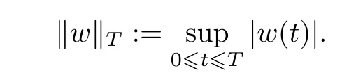
FixT＞0.Letbe the collection of all the continuous functions from[0，T]to Rd.We then equip this with compact uniform convergence topology.Letbe theσ-field generated by the topology.Forw∈，set

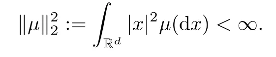
Let B (Rd) be the Borelσ-field on Rd.Let P2(Rd) denote the space of probability measures on B (Rd) with finite second moments;that is，ifμ∈P2(Rd)，then

The distance ofμ1，μ2∈P2(Rd) is defined as

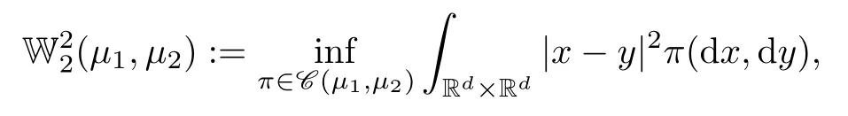
where C (μ1，μ2) denotes the set of all the probability measures whose marginal distributions areμ1andμ2，respectively.Thus，(P2(Rd)，W2) is a Polish space.

Let (Ω，F，{Ft}0≤t≤T，P) be a complete filtered probability space and let{Wt，t≥0}be anm-dimensional standard Brownian motion on it.Consider the following path-dependent MVSDE on Rd:

Hereξis an F0-measurable random vector，θ∈Θ⊂Rlis an unknown parameter，andare Borel measurable.We assume the following:

(H1) There exists a nonnegative constantK1such that，for anyw，v∈，μ，ν∈P2(Rd)，b，σsatisfy

(i)

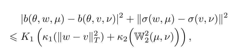
where ‖·‖ denotes the Hilbert-Schmidt norm of a matrix，andκi(x)，i=1，2 are two positive，strictly increasing，continuous concave functions that satisfyκi(0)=0，ε＞0;

(ii)

Theorem 2.1Suppose that (H1) holds and that E|ξ|2＜∞.Then Equation (2.1) has a unique strong solutionXand

ProofFirst of all，set

Step 1We prove that the definition of Equation (2.2) is reasonable.

Forn=0，assume that，forn∈N，

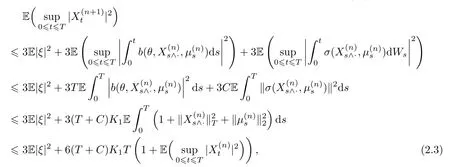
where the last inequality is based on the fact thatFrom induction onn，it follows that

Step 2We prove the existence of the solutions to Equation (2.1).

By deduction the same as to that of (2.3)，it holds that，form，n∈N，

where the last step is based on the Jensen inequality and the fact that

Thus，by[19，Lemma 2.1]，one can getg(T)=0.That is，{X(n)}is a Cauchy sequence in the spaceL2(Ω，F，P，).From this，we know that there exists aX∈L2(Ω，F，P，) such that

Note that

Thus，we conclude that

Then (2.4)，(2.6)，(2.7)，and the dominated convergence theorem imply that，for∀t∈[0，T]，

Therefore，taking the limit on two sides of Equation (2.2) asn→∞，we have that

that is，X·is a solution of Equation (2.1).

Step 3We prove the uniqueness of the solutions to Equation (2.1).

Suppose thatX·and·are two solutions to Equation (2.1).Then，by a calculation similar to that of (2.5)，it holds that

which，together with[19，Lemma 2.1]，yields that

3 The Maximum Likelihood Estimation of Path-Dependent MVSDEs

In this section，we assume (H1).Then Equation (2.1) has a unique solution denoted asXθ.Then we construct a maximum likelihood estimator ofθand prove its properties.LetA*denote the transpose of the matrixA.

Assume the following:

(H2) For anyw∈，μ∈P2(Rd)，(σσ*)(w，μ) is invertible and the system of algebraic equations has (with respect toα(w，μ)) a solution，whereθ0is the true value ofθ.

Next，we study some properties of the maximum likelihood estimatorθT.To do this，we assume the following:

(H3) For anyw∈，μ∈P2(Rd)，b(θ，w，μ) is one-to-one and continuous inθ.

Theorem 3.1(the strong consistency) Under the assumptions (H1)–(H3)，it holds that

ProofSet

Then it holds that，for anyδ＞0，

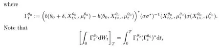
where[·]stands for the quadratic variation of·.Thus，by[10，Theorem 4.6，P.174]，we know that

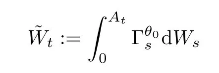
is a (FAt)t≥0-adapted Brownian motion，whereAtis the inverse function ofThus，

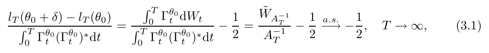
where (H3) is used，and the last step is based on the strong law of large numbers for Brownian motions.By deduction the same as to that of (3.1)，one can get that

Combining (3.1) with (3.2)，we obtain that

Next，we observe (3.3).It follows from (3.3) that，forδandθ0，there exists somet0＞0 such that

Furthermore，by (H3)，we know thatlT(θ) is continuous on[θ0-δ，θ0+δ].Thus，there exists aθ*∈[θ0-δ，θ0+δ]such thatlT(θ*) is the maximum value oflT(θ) on[θ0-δ，θ0+δ].That is，θT=θ*for Θ=[θ0-δ，θ0+δ].Based on (3.4)，it holds thatθTθ0±δforT≥t0.Thus，asT→∞and thenδ→0，θT→θ0.The proof is complete. □

4 The Numerical Simulation of Path-Dependent MVSDEs

In this section，we introduce the numerical simulation of Equation (2.1) under (H1) and estimate the error between the solution of Equation (2.1) and that of the numerical equation under Lipschitz conditions.

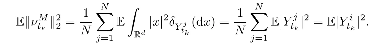
First of all，forN∈N consider the following MVSDEs:

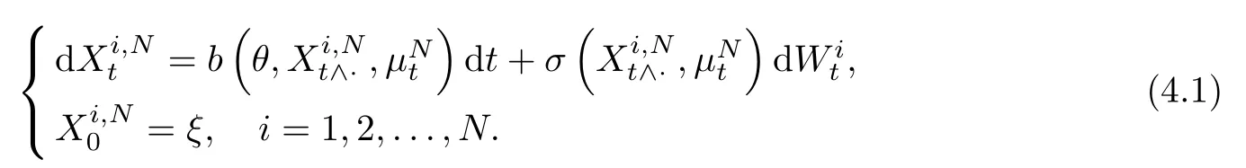
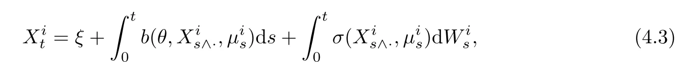
whereis the distribution of.Note that the solution of Equation (4.3) has the same distribution as to that of the solution for Equation (2.1).Therefore，we compute the distance betweento estimate the error betweenXtand.To do this，we need stronger assumptions than (H1).Assume the following:

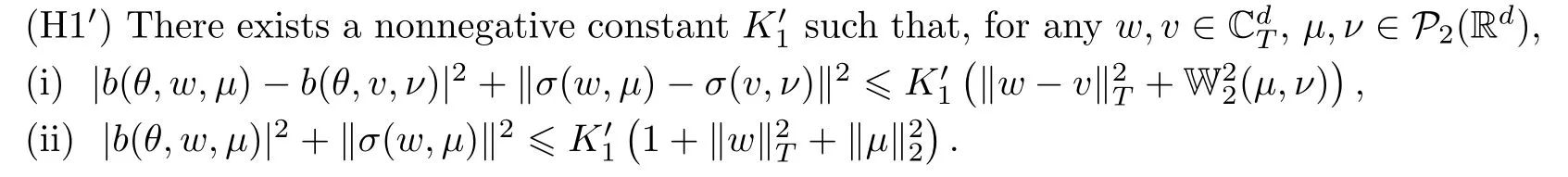
We mention that (i) in (H1′) is a Lipschitz condition.Thus，under (H1′)，it holds that Equation (4.1) has a unique strong solution(see[15]).

Theorem 4.1Suppose that (H1′) holds and that E|ξ|p＜∞forp＞2.Then it follows that

where the constantC＞0 is independent ofN，Mand

ForI1，it follows from deduction the same as to that of (2.5) that，for∀i=1，...，N，

By Gronwall’s inequality，we obtain that

where the last inequality is based on[9，Theorem 1]，and furthermore，

ForI2，by the deduction similar to that of (2.5)，it holds that

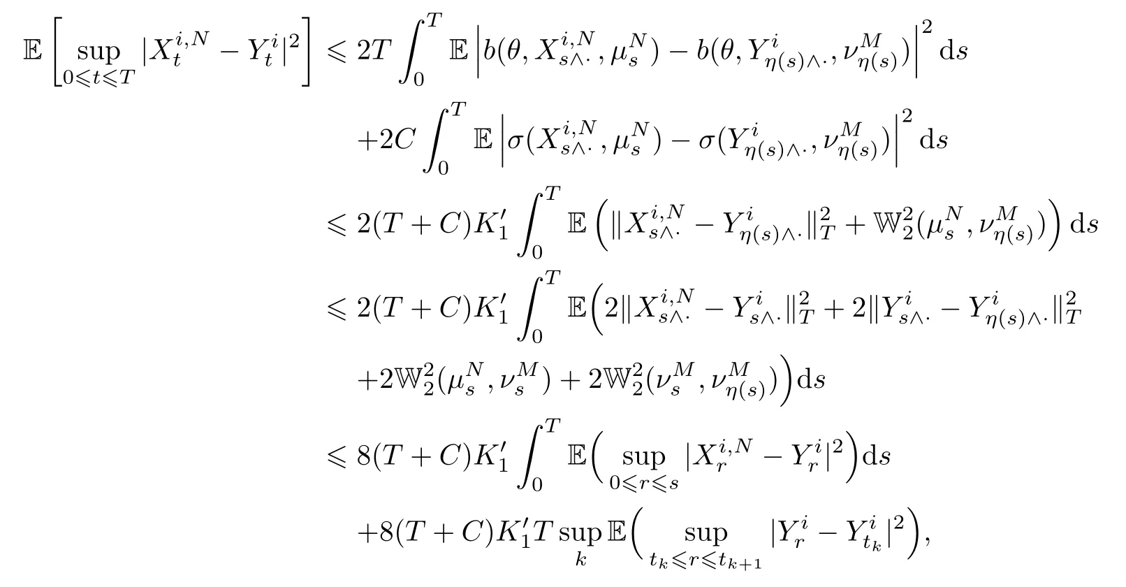
whereη(s)=tk，s∈[tk，tk+1]，and the following fact is used:

Gronwall’s inequality gives us that

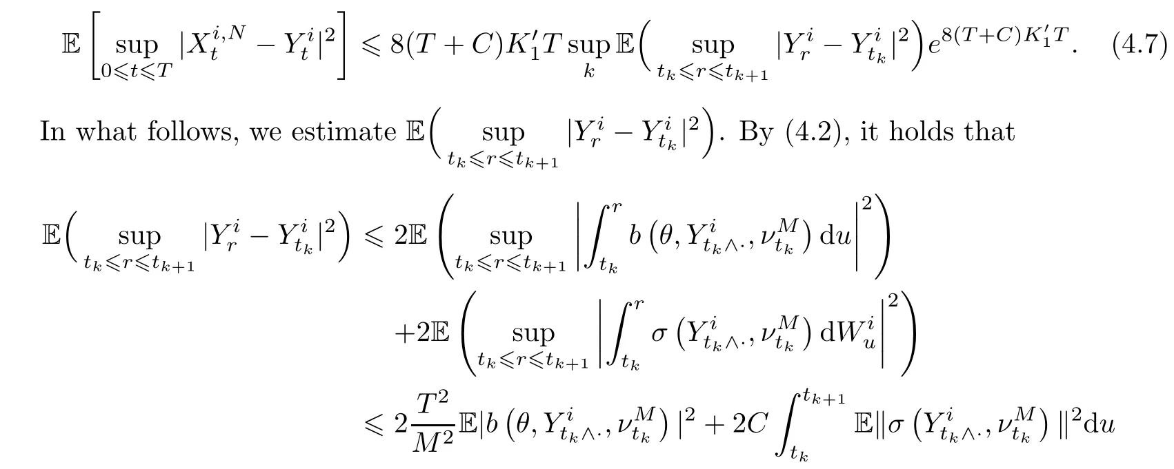
where in the second to last inequality we use the fact that

In addition，from the deduction similar to that of (2.3)，it follows that

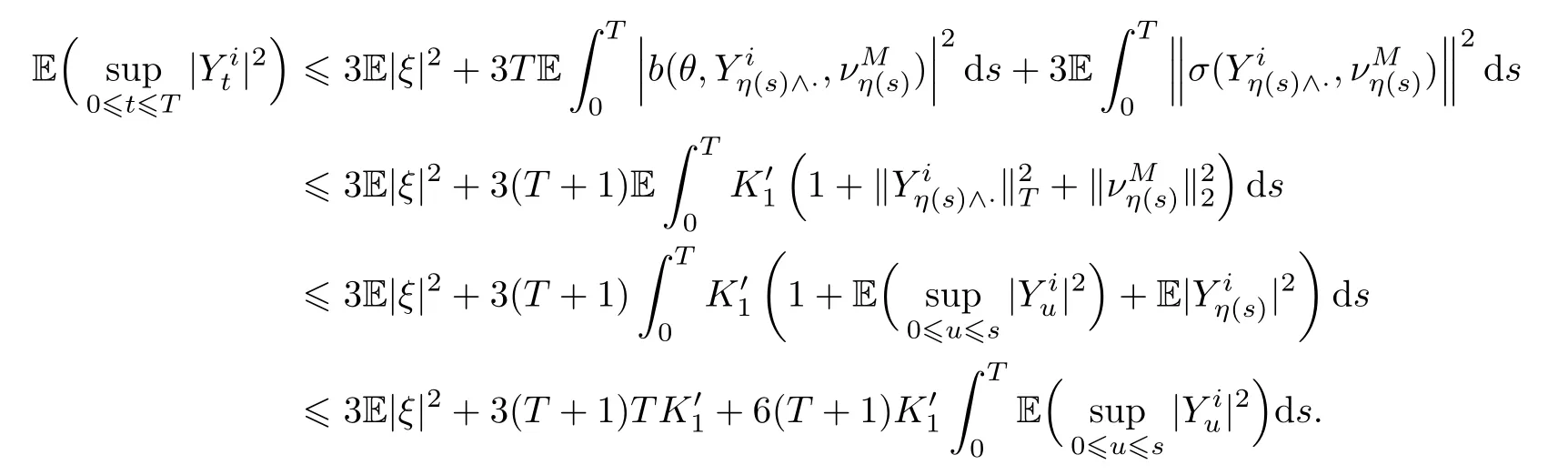
Again by Gronwall’s inequality，we have that

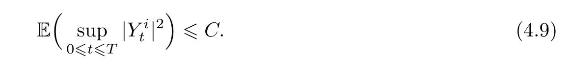
Combining (4.7)–(4.9)，we have that

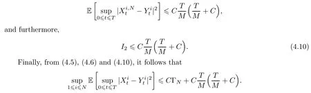
The proof is complete. □

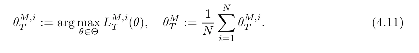
Next，we construct a maximum likelihood estimator of the parameterθ.Assume that (H2) and (H1′) hold.Then define the maximum likelihood function

Thus，the maximum likelihood estimator of the parameterθis given by

AcknowledgementsThe second author thanks Professor Renming Song for providing her with an excellent environment in which to work at the University of Illinois at Urbana-Champaign.Both authors are grateful to the two referees，as their suggestions and comments improved the results and the presentation of this paper.