Inversion method for multi-point source pollution identification: Sensitivity analysis and application to European Tracer Experiment data

Jilin Wng , , Junjun Liu , , , Bin Wng , , Wei Cheng , Jiping Zhng

a The State Key Laboratory of Numerical Modeling for Atmospheric Sciences and Geophysical Fluid Dynamics, Institute of Atmospheric Physics, Chinese Academy of Sciences, Beijing, China

b College of Earth and Planetary Sciences, University of Chinese Academy of Sciences, Beijing, China

c Beijing Institute of Applied Meteorology, Beijing, China

d College of Environmental Sciences and Engineering, Peking University, Beijing, China

Keywords:Source identification Multi-point source pollution Sensitivity analysis European Tracer Experiment

ABSTRACT Fast and accurate identification of unknown pollution sources plays a crucial role in the emergency response and source control of air pollution.In this work, the applicability of a previously proposed two-step inversion method is investigated with sensitivity experiments and real data from the first release of the European Tracer Experiment (ETEX-1).The two-step inversion method is based on the principle of least squares and carries out additional model correction through the residual iterative process.To evaluate its performance, its retrieval results are compared with those of two other existing algorithms.It is shown that for those cases with richer measurements, all three methods are less sensitive to errors, while for cases where measurements are sparse,their retrieval accuracy will rapidly decrease as errors increase.From the results of sensitivity experiments, the new method provides higher estimation accuracy and a more stable performance than the other two methods.The new method presents the smallest maximum location error of 18.20 km when the amplitude of the measurement error increases to 100%, and 22.67 km when errors in the wind fields increase to 200%.Moreover, when applied to ETEX-1 data, the new method also exhibits good performance, with a location error of 4.71 km, which is the best estimation with respect to source location.

1.Introduction

With the increasing occurrence of air pollution and toxic gas leakage incidents, more attention has been given to this area.In these events,rapid and accurate identification of unknown pollutant releases is of vital importance for source control and accurate prediction of subsequent atmospheric transport and dispersion.Source identification generally refers to estimating the number, locations, and intensities of sources from limited concentration measurements and is usually treated as an inversion problem.

The reconstruction of pollutants mainly includes the identification of single ( Allen et al., 2007a ; Keats et al., 2007 ; Thomson et al., 2007 ;Zheng and Chen, 2011 ; Efthimiou et al., 2017 ; Ma et al., 2018 ) or multiple ( Allen et al., 2007b ; Annunzio et al., 2012 ; Sharan et al.,2012 ; Yee, 2008 , 2012 ; Wade and Senocak, 2013 ; Cai et al., 2014 ;Matsuo et al., 2019 ) point sources.For multi-point source identification, on the one hand it is difficult to distinguish the release from each individual source owing to the superposition of multiple concentration plumes, whilst on the other hand the degrees of freedom of the unknowns will increase significantly with the number of sources.Therefore, it makes the inversion problem more complicated and challenging than with single-point source identification.In our previous work, a new two-step inversion method was proposed to address the estimation of multiple releases.Its mathematical consistency has been preliminarily verified with a set of synthetic experiments ( Wang et al., 2021a ).However, the retrieval process may suffer from many uncertainties in the real world.For example, measurement errors are inevitable owing to the inherent accuracy of the sensors or human error, which will undoubtedly cause errors in the final estimation of source parameters.Cai et al.(2014) explored the performance of source reconstruction at three different sensor threshold levels.The results indicated that the identification accuracy of the source intensity tended to decrease with an increase in the sensor threshold.Senocak et al.(2008) analyzed the effect of measurement errors on the retrieval results with noisy synthetic measurements.The noisy measurements were made by adding lognormal distributed noise to the model-generated concentrations.A similar sensitivity analysis was later conducted by Singh and Sharan (2019) , in which a Gaussian distribution was considered.In addition, errors in the wind field, a major driver of atmospheric dispersion, will significantly affect the accuracy of retrieval.Although weather forecasting models have been developed rapidly, the available wind data may still be inaccurate or unrepresentative ( Daley, 1991 ), with insufficient spatial and temporal resolution for the precise modeling of pollutants.To address this issue, Allen et al.(2007a) attempted to determine the surface wind direction along with pollutant source parameters using a genetic algorithm, which further increases the complexity of source estimation.

Considering that the effect of different errors on source reconstruction can be fully understood with sensitivity analysis, two groups of sensitivity experiments were conducted in this study to investigate the robustness of our previously proposed two-step inversion method( Wang et al., 2021a ) with respect to errors in measurements and wind fields.Moreover, an application of the method to real data from the European Tracer Experiment (ETEX) was further performed to verify its practicability in the real world.Accordingly, the structure of this paper is divided into five sections.A brief description of the previously proposed two-step inversion method is given in section 2 , and then the sensitivity analysis and its application to ETEX data are presented in sections 3 and 4 , respectively.Finally, a discussion and conclusions are presented in section 5 .

2.Brief description of the method

The two-step inversion method was preliminarily proposed to solve the problem of multi-point source identification.It can automatically determine the number and locations of sources through an iterative process.In each iteration, the initial guess or the increment of the emission flux is estimated with a simplified optimization algorithm by introducing the weighted influence function.As the iteration proceeds, the initial guess is gradually corrected to the truth.The number and locations of sources can be accordingly determined, and the intensities of all identified sources are further estimated through minimization of the cost function with the least-squares method.For a detailed description of this method, readers are referred to Wang et al.(2021a) .

To evaluate the performance of the two-step inversion method, its retrieval results are compared with those of two other existing algorithms.For convenience, the two-step inversion method studied in this paper is abbreviated as “Method1 ” in the following section.The second algorithm, which iteratively searches all possible grid points and identifies the points with the highest correlation between the observed and simulated concentrations as the source locations ( Wang et al., 2021b ;Efthimiou et al., 2017 ), is called “Method2 ”.Additionally, “Method3 ”refers to the reconstruction of sources by directly minimizing the cost function of the sum of the squared differences between the observed and simulated concentrations with the least-squares method ( Seibert, 2001 ).

3.Sensitivity analysis

In this section, the results of two groups of sensitivity experiments are analyzed to explore the stability of the algorithm with respect to errors in measurements and wind fields.In each group, there were 10 experiments with release scenarios presented in Table 1 .The first four experiments correspond to releases from a single source.The next four cases represent release scenarios involving two-point sources with the same and different source intensities.The last two cases represent situations where three-point releases are considered.The locations of the sources are displayed in Fig.S1.To retrieve the source–receptor relationship (SRR) matrix used for inversion, the Lagrangian particle dispersion model FLEXPART-WRF ( Brioude et al., 2013 ) is utilized.This model has been widely used to simulate the atmospheric transport and dispersion process at meso scales.The simulation setup is consistent with that of Wang et al.(2021a) .In this study, we only focus on the sensitivity of the identification of source locations to errors, because the value of source intensities can be further corrected with the least-squares method if all locations are accurately identified.The indicator of location error (EL),which is calculated as the Euclidean distance between the position of the true source and the center of the identified grid point, is utilized to quantitatively evaluate the performances of the aforementioned three algorithms.The lower the value of the indicator, the more accurate the identification of the point source.

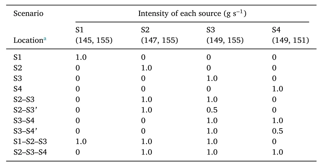
Table 1 The release scenarios of 10 experiments.

3.1. Sensitivity to measurement errors

To represent measurement errors, normally distributed random noise is added to the model-generated concentrations.Perturbations are added in the same manner as described by Wang et al.(2021b) , but in this study the standard deviation of the random noise is chosen to be 30%, 50%, and 100% of the true concentration amplitude.

A total of 500 random disturbances are conducted for each disturbance amplitude, and the averaged results of 500 retrievals are analyzed.Fig.1 displays the estimated location errors for the three methods,where the horizontal coordinates display all sources in 10 different scenarios and the vertical coordinates denote the estimated location error for the respective source.In Fig.1 , the first four groups of bars represent four cases of single-point release (S1, S2, S3, S4); the next four groups are results of four cases for two-point source identification (S2–S3, S2–S3’, S3–S4, S3–S4’); and the last two groups correspond to three-point source cases (S1–S2–S3 and S2–S3–S4).It is observed that the sensitivity to measurement errors differs with different point sources.The retrievals of source S1 and source S2 are more stable than those of source S3 and source S4.This finding is mainly caused by the placement of sensors.As demonstrated in previous studies, e.g., Crenna et al.(2008) , the arrangement of the monitoring network plays an important role in the process of source identification.With the current network, it is found that the monitoring data of point source S1 and source S2 are more abundant and have more peaks, while the peak concentrations of source S3 and source S4 are lower and less.For these cases with scarce measurements, the source term estimation is more susceptible to various kinds of errors.As a result, their retrieval accuracy will decrease rapidly as the measurement noise increases.In addition, it is shown in Fig.1 that all three methods present small location errors at a disturbance amplitude of 30%.When the disturbance increases to 50%, the performance of Method2 gradually worsens, especially for the release scenarios containing source S3 and source S4.For Method2, the maximum location error is approximately 154.37 km, while Method1 and Method3 show a better performance, with smaller maximum location errors of 10.78 km and 20.06 km, respectively (Table S1).As the disturbance increases to 100%, all sources suffer from location errors, and the maximum location error for Method1 has increased to 18.20 km.However, it is obvious in Table S1 that the average location error for Method1 is still the smallest among all three methods.Moreover, to explain the retrieval results, a detailed analysis of the three methods is conducted.This analysis reveals that the higher sensitivity of Method2 to errors is mainly because the algorithm treats the emission as a single point source in each iteration and does not take into account the effects of different grid points.For Method1 and Method3, it is assumed that the releases at all grid points will contribute to the measurements.This consideration makes the algorithms more stable to errors.However, the application of the residual iterative algorithm in Method1 will provide additional model corrections and ultimately produce a more accurate estimation than Method3.Based on the above analysis, Method1 has higher accuracy than Method3 and is more robust than Method2, which makes it ultimately performs better than the other two methods.In conclusion, the three methods can accurately estimate the characteristics of sources in circumstances of small measurement errors; whereas, when the measurement errors increase to a large extent, it is more advantageous to apply the newly proposed two-step inversion method.However, it should be noted that large disturbance amplitudes of 30%–100% are only chosen for the comparison of the robustness of the three methods.Indeed, a disturbance amplitude of 30% is generally enough to represent the measurement noise in the real world, under which all three methods exhibit good behavior.

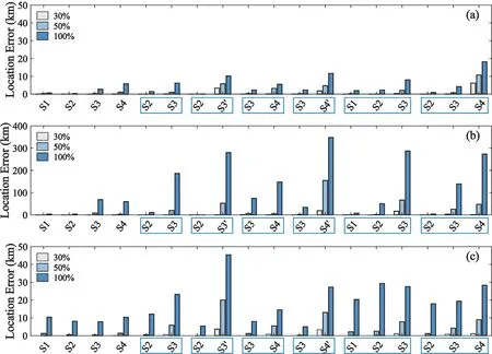
Fig.1.Estimated location errors with noisy measurements: (a) Method1; (b) Method2; (c) Method3.The point sources of each scenario are framed together in blue boxes along the x -axis.

3.2. Sensitivity to wind field errors

The aim of the second group of experiments was to investigate the sensitivity of the three methods to errors in atmospheric wind fields.Considering the Gaussian distribution of wind fields, the zonal and meridional wind components are separately disturbed with normally distributed random noise with a zero mean and standard deviation equal to 50%, 100%, and 200% of their respective standard deviations.

The results of source localization are illustrated in Fig.2 .The location errors exhibit an increasing trend as the disturbance increases from 50% to 200%.For a disturbance amplitude of 50%, all sources are identified with negligible location errors.Subsequently, an error of 7.10 km (approximately 1.5 grid spacing) is found in the estimation of source S3 and source S4 for all methods when the disturbance increases to 100% (Table S2).Furthermore, as the disturbance increases to 200%,the maximum errors of the three methods are 22.67 km, 603.63 km, and 21.29 km, respectively.Consistent with the results of the first group of sensitivity experiments, Method2 estimates source S3 with a large location error because it does not consider the error between grid points.In comparison, the retrieval performances of Method1 and Method3 are more robust with respect to the wind field disturbance, and Method1 has fewer sources with an incorrect estimation and a smaller average location error (Table S2).It is therefore shown that the performance of the two-step inversion method is comparable or even better than that of some previous methods in the presence of wind field disturbance.

4.Application to ETEX data

4.1. ETEX data

Having seen the strong stability of the proposed method with respect to errors in measurements and wind fields, we further explore its application in the real world.The first release of ETEX data (ETEX-1; Nodop et al., 1998 ), which has been widely used in the area of model evaluation and source term estimation, is chosen for validation.In ETEX-1, 340 kg of the non-reactive, non-depositing, non-watersoluble, inert gas perfluorocarbons were constantly emitted at Monterfil ( 48o03′30′′N,2o00′30′′W) , a city in northwestern France.The release started at 1600 UTC 23 October 1994 and lasted for 11 h and 50 min,with an average emission rate of 7.981 g s−1.Air concentrations were sampled at 168 monitoring sites in 17 European countries with a 3-h sampling frequency for approximately 90 h since the initial release.The positions of the release and sampling stations are displayed in Fig.S2.A total of 3104 measurements passed the quality control and were utilized to reconstruct the single source.

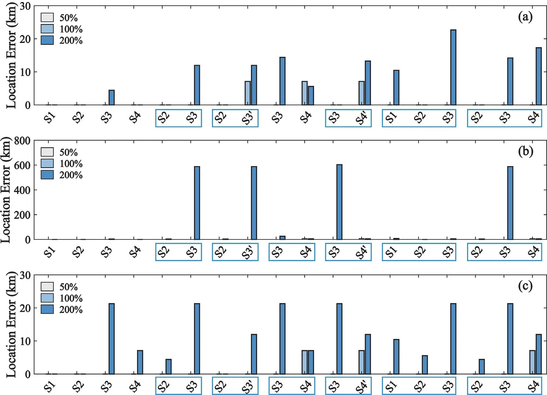
Fig.2.Estimated location errors with perturbed wind fields: (a) Method1; (b) Method2; (c) Method3.The point sources of each scenario are framed together in blue boxes along the x -axis.

4.2. Model setup

In this next part of the study, we report on the use of the FLEXPARTWRF model to retrieve the SRR matrix for inversion.The WRF model was configured with two nested domains of 27 km and 9 km (Fig.S3)to obtain the meteorological input.The physical parameters used in the simulation are summarized in Table S3.Simulations were restarted at 0000 UTC every day and run for 30 h with the first 6 h as a spin-up run.The remaining 24 h were utilized to provide the meteorological fields for FLEXPART.For the simulations of the FLEXPART model, backward runs were made by releasing 500 000 particles from each sampling station at 3-h intervals to retrieve the SRR.The computational domain was configured with a horizontal grid of 351 × 251 and 7 vertical levels, and the SRR was sampled at the lowest layer at a resolution of 0.1° × 0.1°considering the uniform vertical distribution within the boundary layer.

Table 2 Retrieval of the ETEX-1 field experiment for different algorithms.

4.3. Results

The simulation performance of FLEXPART-WRF in ETEX-1 is first examined with a ranking model ( Wade and Senocak, 2013 ).The ranking model can provide an overall score of the simulation results by combining three metrics: scatter (FAC2), bias (FB), and correlation (R2).The metric FAC2 is a measure of error that calculates the fraction of simulations that agree with the observations within a factor of two.In addition,the bias between simulations and observations at the receptors is represented by fractional bias (FB), which can be expressed as

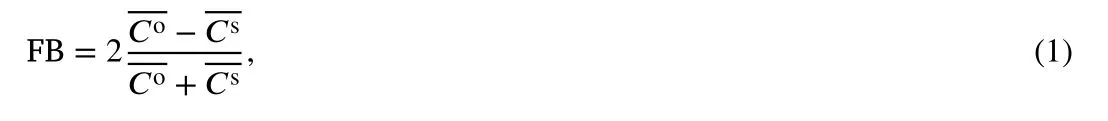
whereCoandCsdenote the average of observations and simulations,respectively.Moreover, Pearson’s correlation coefficient (R) is one of the common indicators reflecting the linear relationship between two variables.It is defined in the form of

wheremis the number of observations andandare the observed and simulated concentrations at theith receptor, respectively.The three statistical parameters mentioned above are combined as shown in Eq.(3) to quantify the accuracy of the simulation:

The composite RANK ranges from 0 to 3, with 3 corresponding to a perfect score.Higher RANK values indicate better performances.For evaluation of the capability of FLEXPART-WRF in ETEX-1, only nonzero observations are used.It achieves satisfactory results, with a high correlation (R2= 0.5853), small bias (FB = 0.4235), and 15.2% of the forecast concentrations within two times the observed values when the true parameters of the source term are provided.The RANK is calculated to be 1.526, showing that the dispersion model can be utilized to simulate realistic atmospheric dispersion in ETEX-1.The spatial distribution of concentrations given in Fig.S4 also reveals high consistency between the observations and simulations.However, it should be mentioned that the model tended to overpredict measurements at the beginning of sampling, especially for the station at Rennes.This problem has also been revealed in Stohl et al.(1998) and may be caused by the model representation error.

Based on the good performance of the FLEXPART-WRF model in ETEX-1, we further utilized the model to retrieve the SRR for point source identification.For emergency responses, accurate localization is particularly crucial.The estimation of source intensity would be meaningless if the source is located at an incorrect position.The reconstructed results related to locations for different algorithms are presented in Fig.S5.It is shown that all three algorithms exhibit good performance.The new two-step inversion method (Method1) provides the best estimation of source location, with the estimation falling at the same grid point as the truth ( Table 2 ).The correlation-based method (Method2) obtains the maximum correlation west of approximately two grid points from its real position, leading to an error of 14.99 km.In contrast, the commonly used least-squares method (Method3) performs the worst in localization,with an error of 23.37 km, approximately three grid points away from the true location.

On the other hand, considering the overprediction of the dispersion model, we try to take the model representation errors into account in the estimation of source intensity.In this study, the error information is statistically calculated with a large number of ensemble samples.A total of 200 000 source intensities are sampled within the specified interval(0–100 g s−1is chosen in this study) so that their corresponding simulations and deviations from measurements can be obtained from the FLEXPART-WRF model run.The standard deviation of these 200 000 simulations is then calculated and treated as error information for each measurement.For quality control, the measurements with a deviation(measurement minus simulation) greater than three times the standard deviation are discarded, and the remaining measurement data are further utilized to estimate the source intensity of ETEX-1 in the second step.With the above method, the source intensities are estimated to be 5.67 g s−1, 7.11 g s−1, and 7.82 g s−1for the three methods, respectively.Overall, the proposed algorithm is proven to perform well in real circumstances, and its retrieval accuracy is comparable to that reported in previous studies, especially for the identification of source locations.

5.Discussion and conclusions

Measurement noise and atmospheric wind field errors may lead to large uncertainties in the practical application of multi-point source identification methods.In this paper, the practicability of the two-step inversion method proposed in our previous study is investigated with two groups of sensitivity experiments and real data from ETEX-1.To evaluate the performance of the proposed method, the results obtained are compared with those of two other existing algorithms.From the results of the sensitivity experiments, all three methods can accurately estimate the number, locations, and intensities of sources when the amplitude of disturbance is small.As the disturbance increases, the superiority of the newly proposed method is gradually highlighted, with smaller location errors.In addition, the method exhibits good performance in the retrieval of ETEX-1, with a location error of 4.71 km.It is the best estimation of source location among the three methods.Furthermore,a detailed analysis of the three methods reveals that all three methods are based on the same principle of least squares, with the difference being that they use different implementations when solving.Compared to Method3, an additional model correction is applied in Method1 through the residual iterative process, which makes the estimation closer to the truth and ultimately produces a more accurate retrieval.Moreover, the residual iterations are applied in Method2 as well.However, Method1 is solved simultaneously for the whole field to obtain the global optimum, while Method2 only considers the error at a single point, and the influence of error between grid points is not considered.In view of this,Method1 and Method2 are approximately equivalent when there are no errors or small errors; whereas, when large errors are considered,the performance of Method1 will be better than that of Method2.Especially for cases with limited measurements, in which retrieval results are more sensitive to various kinds of errors, the new method will be a better choice.In general, the two-step inversion method has advantages in high accuracy and strong robustness with respect to various kinds of errors.This feature makes the algorithm more practical and feasible.However, it should be mentioned that there are still some limitations,such as the lack of consideration of the release height of sources and the ground-level approximation used in source identification.

In addition, it is known that the measurement errors caused by the inaccuracy of the instrument can be statistically determined by the long-term observation bias (observation minus background) of the instrument.This would allow information on the measurement errors to be taken into account in the process of source identification through the utilization of observation error.The cost function of Eq.(3) in Wang et al.(2021a) can therefore be expressed as

whereHis the SRR matrix retrieved from the dispersion model,xis the vector of the source emission to be estimated,Cois the vector of measurements, andRis the observation error covariance, which is usually taken as a diagonal matrix.It should be noted that the matrixRincludes not only the measurement errors but also errors in the calculation of the adjoint functionH(also called the observation operator in the area of data assimilation).Therefore, the errors in wind fields,which will eventually produce errors in the observation operator, can also be represented by the matrixR.The correct estimation of the matrixRwould certainly further improve the accuracy of source identification.

Finally, it is also important to note that the arrangement of the monitoring network has a vital influence on the retrieval results of source identification.When the monitoring data are abundant, the sensitivity of source identification to errors is relatively low; whereas for cases with few measurements, their retrieval accuracy will rapidly decrease as errors increase.Some researchers have pointed out that sensors designed in concentric circles or rows are beneficial in obtaining richer observations and are thus a better estimation of sources.In view of this finding,the construction of a more reasonable and optimal monitoring network will be further discussed in future work.

Funding

This study was supported by the National Key R&D Program of China[grant numbers 2017YFC1501803 and 2017YFC1502102].

Supplementary materials

Supplementary material associated with this article can be found, in the online version, at doi: 10.1016/j.aosl.2021.100147 .