A Feature Weighted Mixed Naive Bayes Model for Monitoring Anomalies in the Fan System of a Thermal Power Plant

Min Wang,, Li Sheng,,Donghua Zhou,, and Maoyin Chen,

Abstract—With the increasing intelligence and integration, a great number of two-valued variables (generally stored in the form of 0 or 1) often exist in large-scale industrial processes.However, these variables cannot be effectively handled by traditional monitoring methods such as linear discriminant analysis (LDA), principal component analysis (PCA) and partial least square (PLS) analysis. Recently, a mixed hidden naive Bayesian model (MHNBM) is developed for the first time to utilize both two-valued and continuous variables for abnormality monitoring. Although the MHNBM is effective, it still has some shortcomings that need to be improved. For the MHNBM, the variables with greater correlation to other variables have greater weights, which can not guarantee greater weights are assigned to the more discriminating variables. In addition, the conditional probability P(xj|xj′,y=k) must be computed based on historical data. When the training data is scarce, the conditional probability between continuous variables tends to be uniformly distributed,which affects the performance of MHNBM. Here a novel feature weighted mixed naive Bayes model (FWMNBM) is developed to overcome the above shortcomings. For the FWMNBM, the variables that are more correlated to the class have greater weights, which makes the more discriminating variables contribute more to the model. At the same time, FWMNBM does not have to calculate the conditional probability between variables, thus it is less restricted by the number of training data samples. Compared with the MHNBM, the FWMNBM has better performance, and its effectiveness is validated through numerical cases of a simulation example and a practical case of the Zhoushan thermal power plant (ZTPP), China.

I. INTRODUCTION

WITH increasing intelligence and integration, a great number of two-valued variables (generally stored as 0 or 1 value) often exist in large-scale industrial processes. For instance, 17381 variables are monitored in the No. 1 generator unit of the Zhoushan thermal power plant (ZTPP), where twovalued variables are more than 8820. These two-valued variables mainly include status monitoring variables and numerical range variables, such as control command signals and vibration over-limit signals, which switch from one state to the other with less influence from process fluctuation noise.

In order to insure the high safety and reliability of largescale industrial processes, the problem of monitoring anomalies becomes more and more important [1]–[5]. The timely and accurate abnormal monitoring can effectively reduce waste of resources, economic losses, and even casualties [6]–[11]. Among a large number of monitoring methods, data-driven techniques have attracted much attention with the advantages of requiring less system information and prior knowledge than model-based and expert experience methods [12]–[19]. For example, principal component analysis (PCA) and its variants have been widely used in industrial processes [20], [21]. In order to detect qualityrelated faults, approaches based on partial least square (PLS)analysis have been proposed [22], [23]. When the training data contains both normal and abnormal working condition samples, linear discriminant analysis (LDA) has been utilized[24]. Kernel dictionary learning can also achieve excellent performance [18]. In addition, many other machine learning methods, such as K-nearest neighbors (KNN) [25], support vector machine (SVM) [26], etc., have also been applied in abnormal monitoring.

However, the fact that two-valued variables ubiquitously exist in large-scale industrial processes presents a challenge to traditional monitoring methods. It is well known that the above mentioned methods are strongly based on continuous variables and may be not suitable for two-value variables. For example, PCA, PLS, LDA, etc. obtain a subspace that is convenient for monitoring through decomposition and then construct statistics or hyperplanes. But, these operations are based on Euclidean distance or Mahalanobis distance, which can not effectively mine the process information of twovalued variables. Two-valued variables are usually deleted during the data preprocessing stage [27], [28]. Recently, the mixed hidden naive Bayesian model (MHNBM) was proposed for the first time to combine both two-valued and continuous variables to improve monitoring performance [28]. Although MHNBM is effective, the variables with greater correlation to other variables have greater weights, which can not guarantee that greater weights are assigned to the more discriminating variables. Moreover, the conditional probabilityP(xj|xj′,y=k)betweenxjandxj′ undery=kmust be computed based on the historical data. When training data is scarce, the conditional probability between continuous variables tends to be uniformly distributed, which will affect performance.

Motivated by the above discussions, a model known as the feature weighted mixed naive Bayes model (FWMNBM) is proposed to overcome the shortcomings of MHNBM. In FWMNBM, the variables that are more correlated to the class have greater weights which results in variables with greater differences under different working conditions contribute more to the model. Meanwhile, FWMNBM can avoid calculating the conditional probability between variables such that it can still be used when there is not enough training data.In addition, a more effective consistent characterization technique is developed for the correlation of mixed variables,and the corresponding feasibility analysis is conducted.Compared with MHNBM, FWMNBM has better performance, and the effectiveness of FWMNBM is validated through the simulations of a numerical example and a practical vibration fault case.

In this paper, the remainder is organized as follows. Some preliminaries are briefly outlined in Section II. In Section III-A,FWMNBM is elaborated on. The estimation of parameters is introduced in Section III-B. In Section IV, the effectiveness of FWMNBM is verified. Finally, conclusions are drawn in Section V.

II. PRELIMINARY

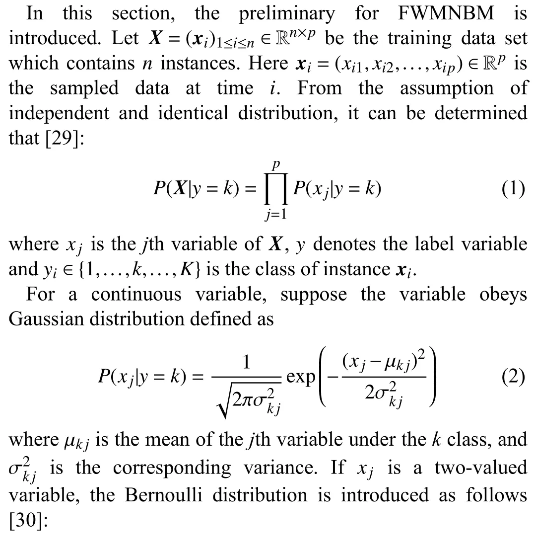
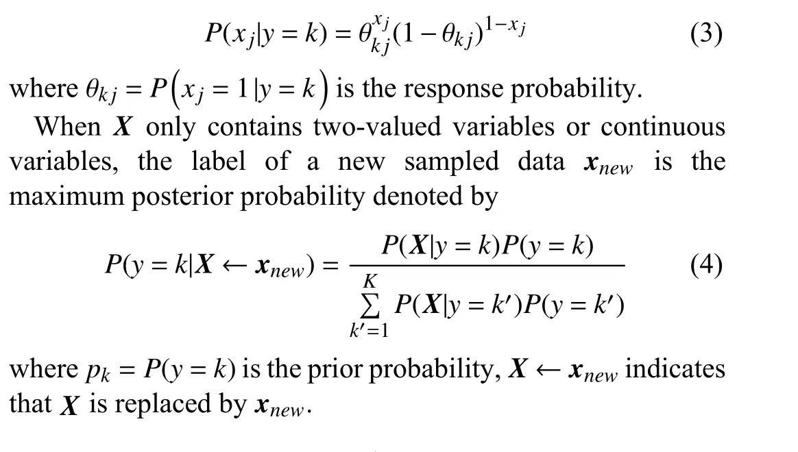
III. MAIN ALGORITHM

A. FWMNBM

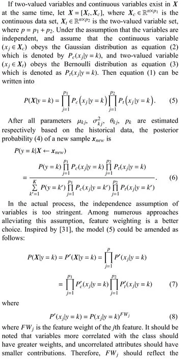
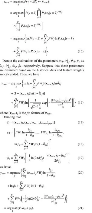
correlation between thexjandyas accurately as possible. The mutual information (MI)MI(xj,y) is used to characterize the correlation betweenxjandy.MI(xj,y) can effectively describe the correlation betweenxjandy, but it also contains some correlational information betweenxjand other variables(such asxj′) because variables are coupled. Then, the average feature-feature intercorrelation is introduced to compute the feature weight [32]

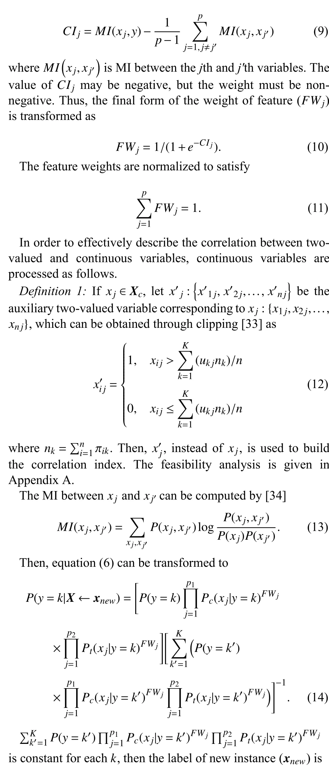
B. Parameters Estimation

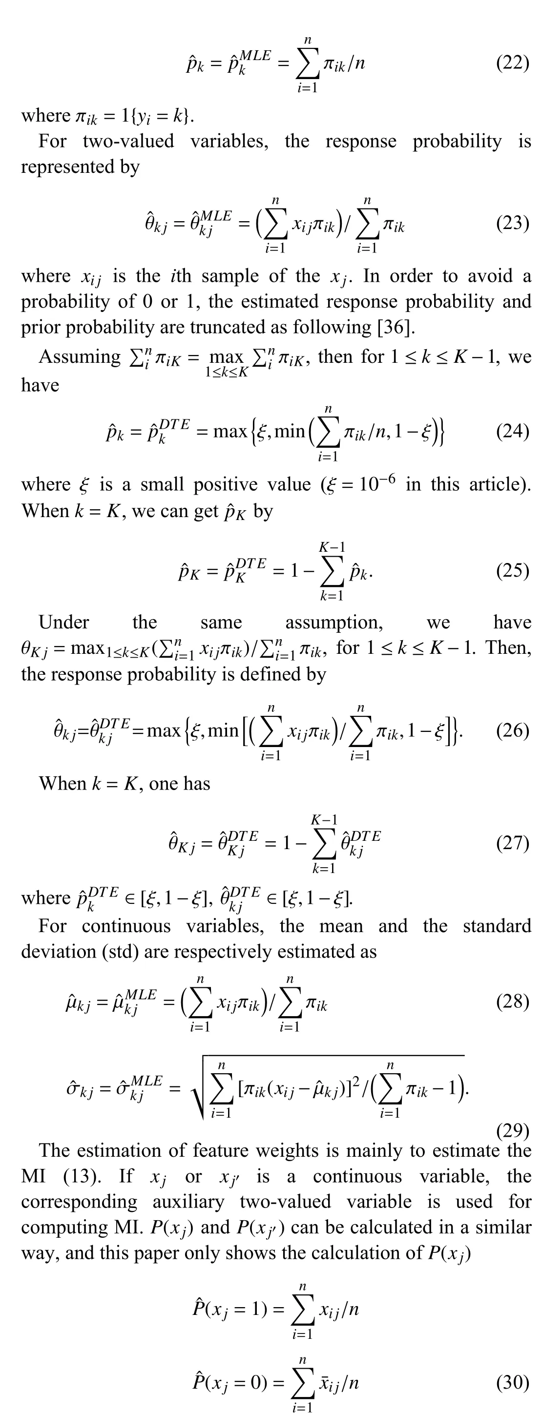
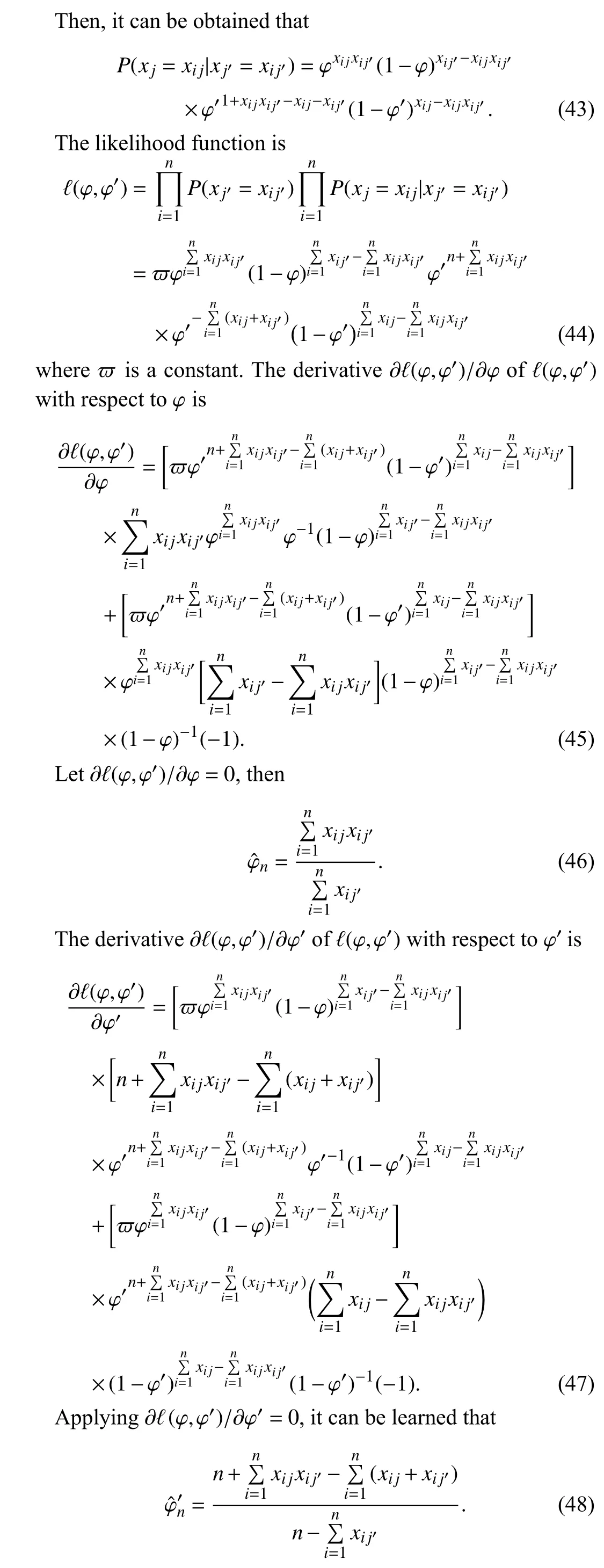
In this subsection,Xis used for parameter estimation.According to maximum likelihood estimation (MLE) [35], the prior probability can be given as

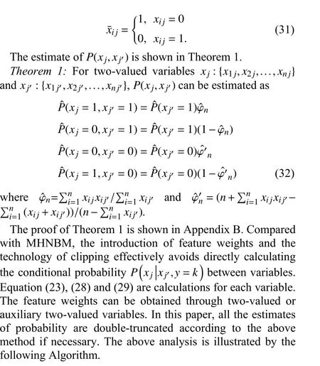
where

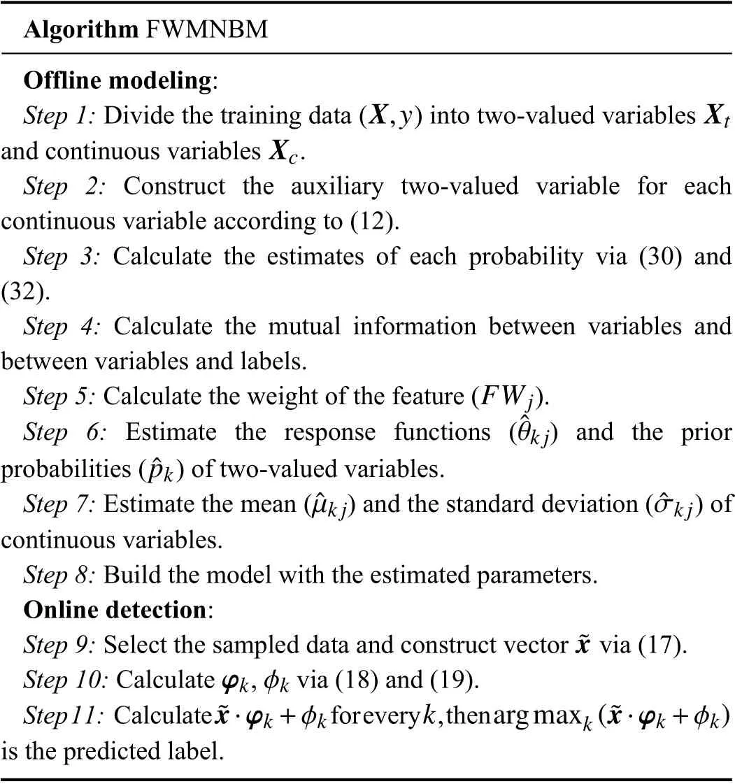
Algorithm FWMNBM Offline modeling:X,yXt Xc Step 1: Divide the training data () into two-valued variables and continuous variables .Step 2: Construct the auxiliary two-valued variable for each continuous variable according to (12).Step 3: Calculate the estimates of each probability via (30) and(32).Step 4: Calculate the mutual information between variables and between variables and labels.FWj Step 5: Calculate the weight of the feature ().ˆθk j ˆpk Step 6: Estimate the response functions ( ) and the prior probabilities ( ) of two-valued variables.ˆµk jˆσk j Step 7: Estimate the mean ( ) and the standard deviation () of continuous variables.Step 8: Build the model with the estimated parameters.Online detection:˜x Step 9: Select the sampled data and construct vector via (17).φkφk Step 10: Calculate , via (18) and (19).˜x·φk+φkkargmaxk(˜x·φk+φk)Step 11: Calculate for every , then is the predicted label.

IV. SIMULATION

In this section, the numerical cases of a numerical simulation example and a practical vibration fault case of ZTPP are utilized to validate the effectiveness of FWMNBM.

A. Numerical Simulation

The numerical simulation data contains 5 continuous variables and 5 two-valued variables. The means of continuous variables are shown in Table I and corresponding standard deviations (stds) are displayed in Table II. The twovalued variable values under different classes are depicted in Table III. In order to make the case more general, the twovalued variable values under different classes are randomly adjusted. The adjustment percentages are listed in Table III.For instance, some values ofv6under normal working conditions, which are set as 0, are changed to be 1 after adjusting. Under each working condition, 1500 samples are randomly generated according to the parameters. The samples under normal 1 and fault 1 are used for training the model,and the other instances are used for testing.

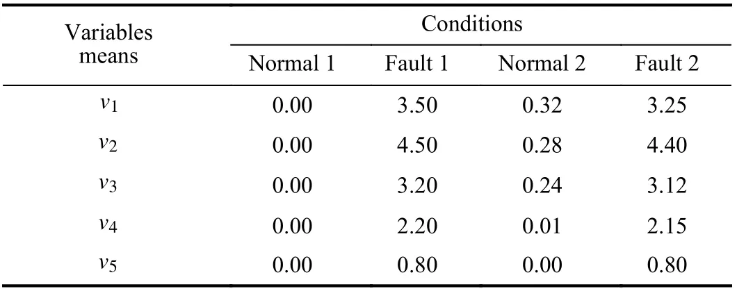
TABLE I THE PRESET MEANS OF CONTINUOUS VARIABLES

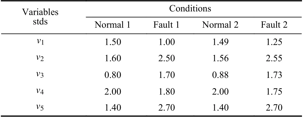
TABLE II THE PRESET STDS OF CONTINUOUS VARIABLES

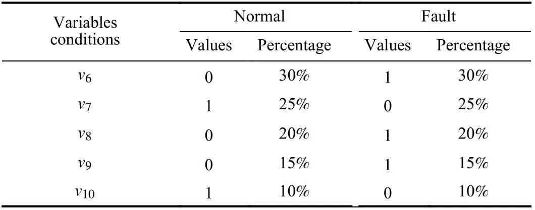
TABLE III THE VALUES AND ADJUSTMENT PERCENTAGE OF TWO-VALUED VARIABLES

The Gaussian naive Bayesian model (GNBM) is used for the continuous variables and the Bernoulli naive Bayesian model (BNBM) is utilized to two-valued variables. That is onlyv1,...,v5are used for build and test GNBM, and BNBM just utilize the information ofv6,...,v10for modeling and verification. Different from GNBM and BNBM, MHNBM and FWHNBM are utilized for modeling and anomaly detection with both two-valued and continuous variables. The first 1500 samples of test data are normal data, and the rest are marked as faults. The test results of all above models for the testing data are depicted in Figs. 1(a)–1(d). There are a lot of false alarms and missing faults when only continuous or twovalued variables are used, which can be seen in Figs. 1(a) and 1(b). MHNBM and FWHNBM have better performance because they can simultaneously mine continuous and twovalued information at the same time. Compared to MHNBM,FWHNBM has the lower false alarm rate (FARs) and a higher fault detection rate (FDR) which are depicted in Figs. 2(e) and 2(f).

B. Actual Data Validation

A vibration fault of ZTPP is also used to illustrate the effectiveness of FWMNBM. At 11:35 on September 3, 2017,a hydraulic cylinder vibration fault of the primary air fan occurred, and it was recovered after 26 hours. The data,containing 495 two-valued variables and 260 continuous variables, is sampled every 5 seconds and collected from 11:35, September 1, 2017. A total of 53280 instances are collected for model training and testing.

The first 60% instances under normal conditions and first 60% fault instances are utilized for modeling, and the remaining data is used for testing. In this article, we used 35 two-valued variables and continuous variables respectively.The detailed variable selection process can refer to article[28]. In the traditional methods, LDA [24], decision trees(DT) [37], SVM [26], k-nearest neighbors (KNN) [25] are adopted to detect anomaly with the continuous variables.MHNBM and FWMNBM are used with both two-valued and continuous variables. The testing results of all methods are shown in Figs. 2(a)–2(f).

Excepting for DT, the performance of other methods in terms of FDR are very satisfactory. DT has omission of fault and all methods have false alarms. In order to compare the performance of various methods, the FDRs and FARs of all methods are shown in Table IV. From the experimental results, the addition of two-valued variables can reduce the impact of parameter fluctuations before a fault occurs.Affected by anomaly evolution, some normal instances are misclassified into fault. However, MHNBM and FWMNBM effectively reduce FAR through combining multiple process data sources, because the advantages of both two-valued and continuous variables are taken into consideration. Among all methods, FWMNBM has the best detection performance.

V. CONCLUSIONS

A data-driven anomaly detection method called FWMNBM is proposed with both two-valued and continuous variables.For FWMNBM, the variables more correlated to class have greater weights, which makes the more discriminating variables contribute more to the model. At the same time,FWMNBM can effectively avoid calculating the conditional probability between variables so that it can still be used when the amount of training data is not sufficient. In addition, a more effective consistent characterization method for the correlation of mixed variables is provided, and the corresponding feasibility analysis is conducted. The superior performance of FWMNBM is verified by the numerical cases of a numerical simulation example and an actual plant’s case.Compared to traditional classical approaches, MHNBM and FWMNBM significantly improve the anomaly monitoring performance by increasing the information of two-valued variables. Furthermore, FWMNBM has more outstanding performance because greater weights are assigned to variables with greater difference under different working conditions.

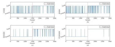
Fig. 1. The label results of different methods. (a) GNBM; (b) BNBM; (c) MHNBM; (d) FWMNBM.

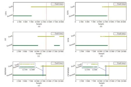
Fig. 2. The testing results. (a) LDA; (b) KNN; (c) DT; (d) SVM; (e) MHNBM; (f) FWMNBM.

APPENDIX A ANALYSIS OF DEFINITION 1

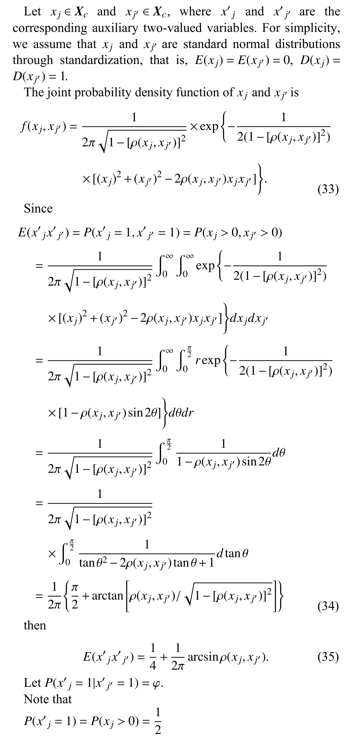
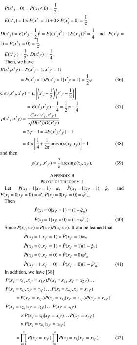
Definition 1 unifies the correlation analysis between variables containing both two-valued and continuous variables by the same standard. The correlation between two-valued variables and two-valued variables or between continuous variables and continuous variables can be effectively characterized, and the original two-valued variables do not change. Therefore, the rationality of Definition 1 can be proved when a quantitative relationship exists between the correlation index of the auxiliary two-valued variables and that of original continuous variables.

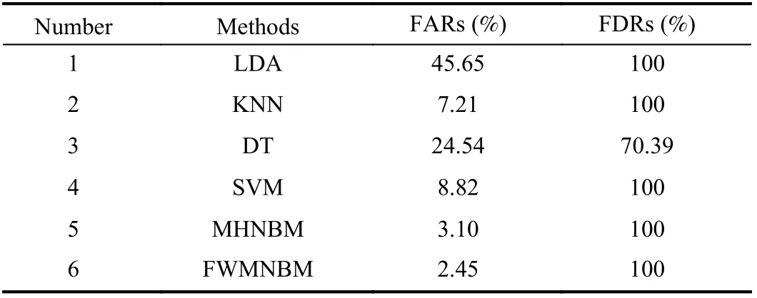
TABLE IV FARS AND FDRS OF ALL METHODS