Recursive Least Squares Identification With Variable-Direction Forgetting via Oblique Projection Decomposition
2022-01-26KunZhuChengpuYuandYimingWan
Kun Zhu,Chengpu Yu,and Yiming Wan
Abstract—In this paper,a new recursive least squares (RLS)identification algorithm with variable-direction forgetting (VDF)is proposed for multi-output systems.The objective is to enhance parameter estimation performance under non-persistent excitation.The proposed algorithm performs oblique projection decomposition of the information matrix,such that forgetting is applied only to directions where new information is received.Theoretical proofs show that even without persistent excitation,the information matrix remains lower and upper bounded,and the estimation error variance converges to be within a finite bound.Moreover,detailed analysis is made to compare with a recently reported VDF algorithm that exploits eigenvalue decomposition (VDF-ED).It is revealed that under non-persistent excitation,part of the forgotten subspace in the VDF-ED algorithm could discount old information without receiving new data,which could produce a more ill-conditioned information matrix than our proposed algorithm.Numerical simulation results demonstrate the efficacy and advantage of our proposed algorithm over this recent VDF-ED algorithm.
I.INTRODUCTION
RESEARCH on system identification dates back to the 1960s,but is still very active due to its critical importance in systems and controls [1],[2].For online parameter estimation,recursive least squares (RLS) identification is one of the most well-known methods [3].To enhance tracking capability of time-varying parameters,exponential forgetting(EF) was initially established for RLS identification of singleoutput (SO) systems,which discounts old information with a constant forgetting factor [3].Various RLS extensions with or without EF have been proposed for multiple-output (MO)systems that are ubiquitous in industrial applications [4]–[11].The parameter errors given by the EF algorithms exponentially converge if the identification data is persistently exciting[12],[13].However,the condition of persistent excitation cannot be always satisfied in practice.With non-persistent excitation,the EF algorithm discounts old data without receiving sufficient new information.As a result,the undesirable estimator windup phenomenon occurs,i.e.,the RLS gain grows unbounded,and the obtained estimates become highly sensitive to noise.
The above limitation of EF in the absence of persistent excitation is attributed to discounting old information uniformly over time and in the parameter space.To cope with this issue,various modified forgetting strategies have been reported in the literature,which can be classified into two categories: Variable-rate forgetting (VRF) and variabledirection forgetting (VDF).The category of VRF algorithms adjusts a variable forgetting factor to discount old information non-uniformly over time.For example,the forgetting factor is updated according to the prediction error [14],[15] by minimizing the mean square error [16] or in accordance with Bayesian decision-making [17].Convergence and consistency of a general VRF algorithm was recently investigated in [18].However,data excitation in practice is not uniformly distributed over space,but might be restricted to certain directions of the parameter space over a period of time.In this case,the VRF algorithms still gradually lose information in the non-excited directions,which would lead to illconditioned matrix inversion and increased estimation errors[19].This problem is addressed by the VDF algorithms in[19]–[21].Specifically,forgetting is applied only to directions that are excited by the online data.By doing so,estimator windup does not occur under non-persistent excitation,because information in the non-excited subspace is retained.
The VRF and VDF algorithms were initially proposed for SO systems.Considering MO systems,the VRF algorithm is still applicable since it simply applies uniform forgetting to the entire parameter space [18],[22].However,the extension of VDF algorithms to cope with MO systems is not straightforward,since the forgotten subspace varies with the online data.As the latest progress in this line of research,a VDF algorithm via eigenvalue decomposition (VDF-ED) has been proposed in [23],[24] for MO systems.The basic idea is to apply forgetting to the eigendirections of the old information matrix where new information is received.Moreover,this VDF-ED algorithm is combined with a variable forgetting factor to further enhance its tracking performance [24].
In this paper,a new VDF algorithm using oblique projection decomposition (VDF-OPD) is proposed for MO systems under non-persistent excitation.Oblique projection is exploited to decompose the old information matrix into a forgotten part and a retained part.This proposed VDF-OPD algorithm has three main contributions:
1) The proposed decomposition of the information matrix has a clear geometrical interpretation based on oblique projection.It reduces to the decomposition described in [21]when the considered system has a scalar output.
2) A detailed comparison with the recently proposed VDFED algorithm in [23] is provided.The forgotten subspace in the VDF-ED algorithm has a higher dimension than that in our VDF-OPD algorithm.Under non-persistent excitation,the VDF-ED algorithm produces a more ill-conditioned information matrix,because part of its forgotten subspace discounts old information without receiving new data.
3) Boundedness of the information matrix and convergence of the estimation error variance of our VDF-OPD algorithm are proved under non-persistent excitation.
The rest of this paper is organized as follows.Firstly,Section II states the problem of RLS identification of MO systems under non-persistent excitation.Our proposed VDFOPD algorithm is presented in Section III,and compared with the VDF-ED algorithm in Section IV.Then,Section V gives the convergence analysis.Finally,simulation results and concluding remarks are provided in Sections VI and VII,respectively.
Notations: The 2-norm of a vectorxis denoted by ‖x‖.For a matrixX,R ange(X),N ull(X),‖X‖2,andX†represent its range space,nullspace,induced 2-norm,and Moore-Penrose inverse,respectively.For a square matrixX,tr(X) denotes its trace,and λmin(X) and λmax(X) represent its minimal and maximal eigenvalues,respectively.For a symmetric matrixX,the positive definiteness and positive semi-definiteness are denoted byX>0 andX≥0,respectively.LetInrepresent an identity matrix of dimensionn.The vectorization operator vec(X)creates a column vector by stacking the columns vectors of a matrixX.For matricesXandY,diag(X,Y)represents a block-diagonal matrix whose diagonal blocks areXandY.
II.PROBLEM STATEMENT
Consider the following MO system [25]
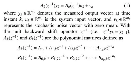
which include slowly time-varying parameters in their coefficient matrices.Define

with Θk∈Rn1×my,φk∈Rn1.Then,the system model (1) is written into

where the parameter vector θkand the regressor matrix Φkare defined as

To estimate the parameter vector θkin (3),the standard RLS algorithm with EF is [22]

The above EF algorithm works well if the regressor sequence {Φk} is persistently exciting [12],[13],i.e.,there exist α >0 and a positive integers0such thatholds for allk>0.The persistently exciting data contains rich new information to compensate for discounted old data.However,under non-persistent excitation,the old information inRkcould be discounted continuously without being fully replaced by any new information from Φk.As a result,some eigenvalues ofRktend to be zero,and the corresponding gainbecomes unbounded,i.e.,the undesirable estimator windup occurs.In this situation,the obtained parameter estimates become highly sensitive to noise.
To address the estimator windup under non-persistent excitation,various VDF strategies have been reported in the literature for SO systems [19]–[21].However,these VDF algorithms consider only aregressor vector,thus cannot cope with the regressor matrix Φkfor MO systems.In this paper,we propose the VDF-OPD algorithm for MO systems,analyze its benefit over the VDF-ED algorithm recently reported in[23],and investigate its convergence properties.
III.RLS WITH VARIABLE-DIRECTION FORGETTING VIA OBLIQUE PROJECTION DECOMPOSITION
For the RLS identification,the basic idea of VDF is to apply forgetting only to directions that receive new information[21].Following this idea,(5b) is modified by decomposing the old information matrixRk-1into two disjoint parts as

In the following derivations,we assume Φk≠0 andRk-1>0.Note thatRk-1>0 will be proved later in Theorem 3.For MO systems,the following requirements are imposed for the decomposition in (6):
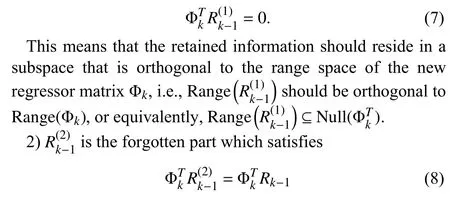
according to (6) and (7).This means that the forgotten partand the old information matrixRk-1have the same amount of correlation with Φk.
3) The two decomposed parts are disjoint,i.e.,

4) Positive semi-definiteness,i.e.,

Geometrically,the above requirements can be satisfied by applyingoblique projectiontoRk-1.Definetwo complementary subspaces,satisfying
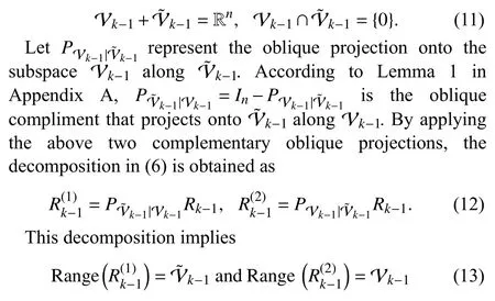
sinceRk-1is non-singular.Then,requirements (7)–(9) for the above decomposition are satisfied by setting

according to Lemma 1 in Appendix A.As indicated by (13),are the forgotten and retained subspaces,respectively.
It is reasonable to require that information in the entire subspaceis all retained,i.e.,

Otherwise,certain directions within Null() would be included in the forgotten subspace Vk-1,and old information in those directions would be discounted without being compensated by new information from Φk.
Being a complement subspace of V˜k-1,Vk-1is to be determined such that,as required in(10).For this purpose,one solution is

a ndthe corresponding oblique projection matrix ontoVk-1alongis
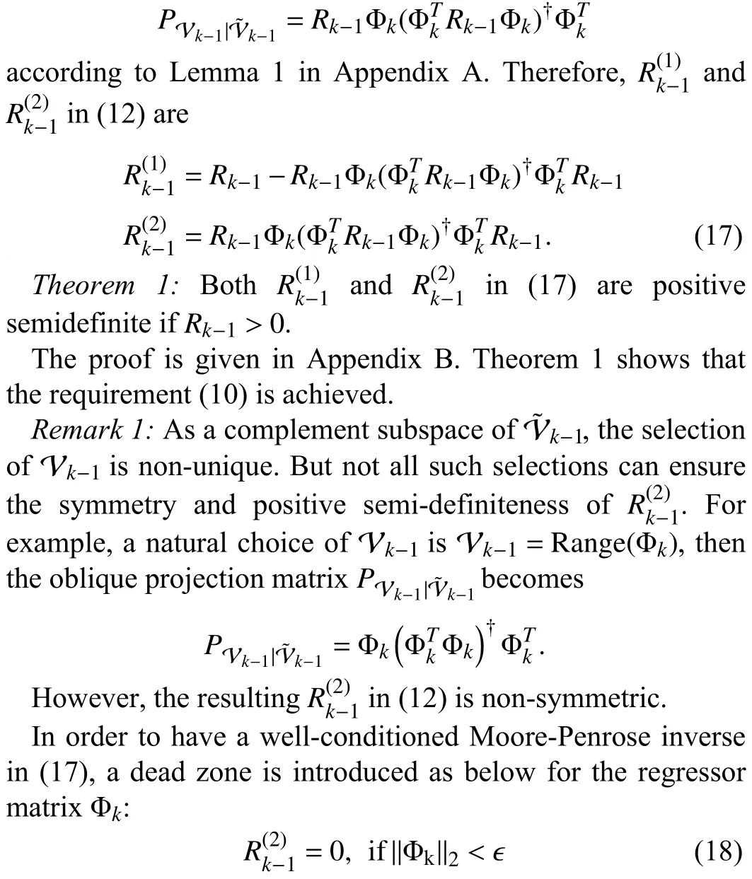
whereϵis determined by the noise level in the data.If Φklies in the above dead zone,Φkis dominated by noise and carries little new information.In this case,the VDF algorithm should not forget any old information inRk-1,and the decomposition(6) is not performed.
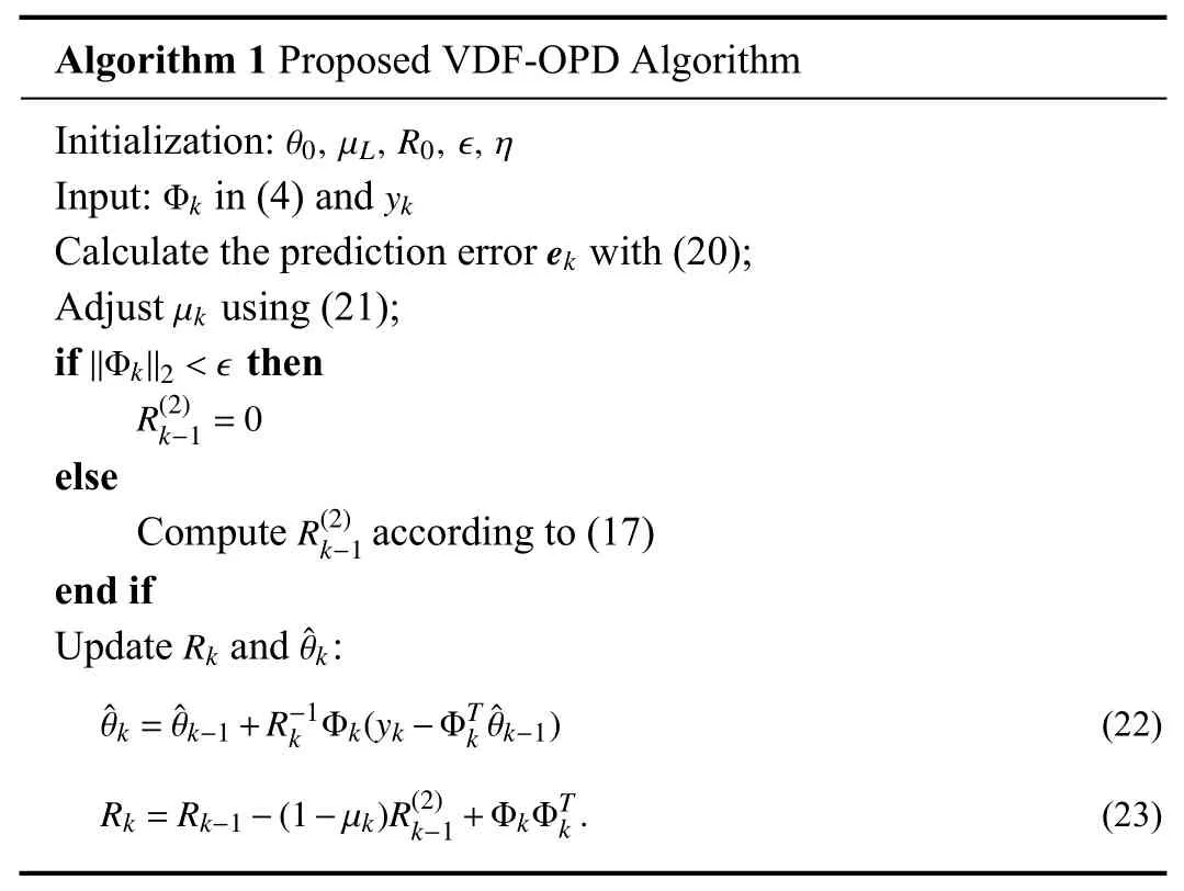
By applying a variable forgetting factor μkonly to,the information matrixRkis updated by

The variable forgetting factor μkis introduced to further improve tracking capability of the proposed VDF-OPD algorithm.Various VRF strategies,such as those found in[14]–[16],can be used to update μkadaptively.In this paper,μkis adjusted according to the prediction error


where μLrepresents the lower bound of μkandηis a positive constant chosen by the user.The user-defined constantηcan be viewed as a sensitivity factor: a smallerηleads to higher sensitivity of μkto variations ofek.As can be seen from (21),when the prediction errorekincreases,a smaller forgetting factor is used such that the parameter estimate tracks the timevarying parameters at a faster rate.
The above proposed VDF-OPD algorithm is summarized in Algorithm 1.Note that (23) is derived from (19) and (6).When the considered system (1) has only a scalar output,the regressor Φkdefined in (4) becomes a vector,and Algorithm 1 reduces to the one proposed in [21].
IV.COMPARISON WITH VARIABLE-DIRECTION FORGETTING VIA EIGENVALUE DECOMPOSITION
Recent progress made in the VDF-ED algorithm in [23] is applicable to MO systems,thus is closely related to our VDFOPD algorithm.However,theoretical analysis of VDF-ED in[23] considers only the condition of persistent excitation,e.g.,see Proposition 10 in [23].Then,it is of interest to compare these two VDF algorithm under non-persistent excitation.
In the VDF-ED algorithm,the information matrixRkis updated by [23]
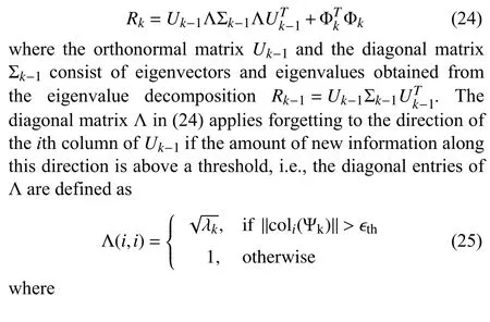

coli(Ψk) is theith column of Ψkthat represents the information content of the regressor matrix Φkalong theith column ofUk-1,λk∈(0,1) is the forgetting factor,and ϵthis a user-defined scalar which should be larger than the noise level.
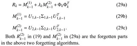
To facilitate the following analysis,according to (25),is rewritten as

where bothU1,k-1andU2,k-1consist of columns ofUk-1,and satisfy

respectively.With (24) and (25),the old information in Range(U1,k-1)is retained,while the old information in Range(U2,k-1)is forgotten.Therefore,the information update in (24) and (25) can be expressed in a form similar to (19),i.e.,
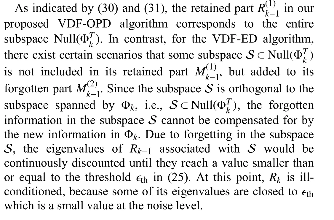
Theorem 2:AssumeRk-1>0.Consider the noise-free case.Set ϵ=0 in (18) and ϵth=0 in (25).Our proposed VDF-OPD algorithm differs from VDF-ED in the adopted two decompositions (17) and (29),i.e.,

The proof is given in Appendix C.In the noisy case,we still have (30) and (31) if the amount of informative data in Φkis significantly larger than noise,and the corresponding proof follows the same idea in Appendix C but with more tedious derivations.
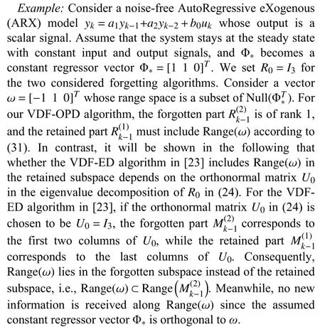
It should be also noted that the orthonormal matrixUk-1in(24) is non-unique ifRk-1has identical eigenvalues.A different selection of eigenvectors inUk-1might result in a different decomposition ofRk-1in (29).For instance,in the above example,if we choose the two retained subspaces in VDF-OPD and VDF-ED are identical,i.e.,the range space spanned by the last two columns ofU0given above.This issue caused by the non-unique orthonormal matrixUk-1in (24) does not occur in our VDFOPD algorithm.

V.CONVERGENCE ANALYSIS
In this section,the convergence behavior of our proposed VDF-OPD algorithm under non-persistent excitation is investigated.
For this purpose,it is important to first analyze the boundedness of the information matrixRkat all time instants[21].With a lower boundedRk,the algorithm gainremains upper bounded,which prevents the estimator windup phenomenon.With an upper boundedRk,the algorithm gaindoes not approach zero,thus it retains its tracking capability.The following two theorems show thatRkis bounded from below and above without requiring persistent excitation.In contrast,the VDF-ED algorithm in [23] only analyzes the lower bound ofRkunder persistent excitation,while the VDF algorithm in [21] is not applicable to MO systems in this paper.
Theorem 3:Consider the recursive update ofRkin (23).Withϵdefined in (18),ifR0>0 and ε ≤‖Φk‖2<∞ for allk>0,then 1)for μk>0 andk>0; and 2) there exists βk>0 such thatRk>βkInfor allk>0.
Theorem 4:With ϵ defined in (18),assume ε ≤‖Φk‖2<∞ at allk>0 .Then,there exist a finite constant γ >0 such thatRk<γInfor allk>0.
Proofs of Theorems 3 and 4 are given in Appendices D and E,respectively.
To analyze the dynamics of parameter estimation errors,we assume θkin (3) to be constant,as in [19],[23].Letθrepresent the true constant parameter.Then,the estimation error is defined by

The following theorem shows that in the presence of noise,the estimation error variance converges to be within a finite bound.
Theorem 5:Withϵdefined in (18),assumeε <‖Φk‖2≤∞,∀k>0.Define

There exista∈(0,1) andb∈(0,1) such that
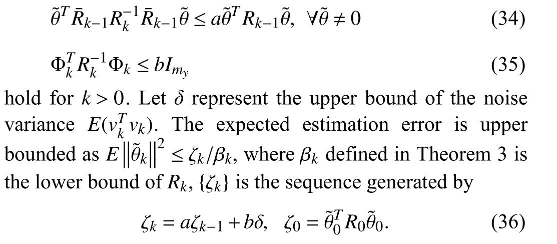
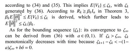
The bounding sequence { ζk} converges to ζ∞=bδ/(1-a) askgoes to infinity,and monotonically decreases if ζk>ζ∞.
The proof is given in Appendix F.
Remark 2:The convergence property holds only when the parameter is constant or its change rate is slower than the algorithm’s convergence speed.
VI.SIMULATION STUDY
In this section,we present a numerical example to show the efficacy of our proposed VDF-OPD algorithm and its advantage over the VDF-ED algorithm in [23].
The identification data is generated by the following MO system

whose parameters and input signals are
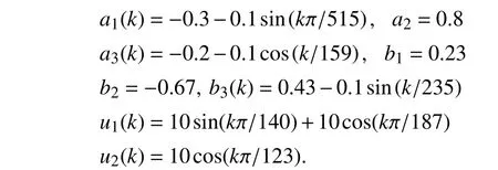
This system model is equivalently written as

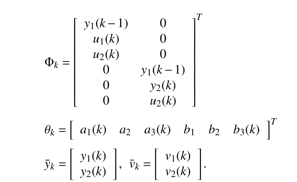
The measure noisevkis Gaussian,with zero mean and covariance matrix 0 .01I2.
Three RLS algorithms are implemented for comparisons:the EF algorithm,our proposed VDF-OPD algorithm,and the VDF-ED algorithm in [23].In all three implemented algorithms,the initial guess of the parameter is=[0.50.50.5 0.50.5 0.5]T,andtheinitialinformation matrix isR0=10-3I6.The constantforgetting factorμinEFis 0.95,while the VDF-OPD and VDF-ED algorithms use the same variable forgetting factor strategy in (21) withη=10-2and μL=0.5.The thresholdsϵin (18) and ϵthin (25) are both set to 0.1.
The parameter estimates from the two VDF algorithms are depicted in Fig.1,while those given by EF are shown in Fig.2.The achieved estimation performance listed in Table I is evaluated by root mean square error (RMSE) of each element in θk,i.e.,
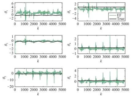
Fig.2.The estimation results of EF algorithm.

where θk(i) and(i) represent theith element of the true parameter and its estimate at timek,respectively.
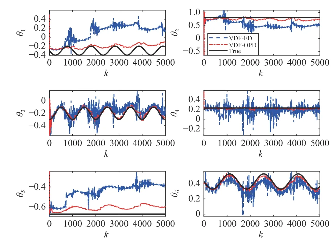
Fig.1.The estimation results of two VDF algorithms.
As indicated by Fig.2 and Table I,the parameter estimates from the EF algorithm have the largest errors,and our proposed VDF-OPD algorithm gives the smallest estimation errors.This can be explained by the evolution of the minimal eigenvalue of the information matrixRk,i.e.,λmin(Rk),in these algorithms,as depicted in Fig.3.For the EF algorithm,its λmin(Rk) is significantly smaller than the other two algorithms,hence its obtained estimates are most sensitive to noise.After about time instantk=700,the VDF-ED algorithm gives highly noisy estimates in Fig.1,because its value of λmin(Rk) decreases to around 0.1.Compared to EF and VDF-ED,our VDF-OPD algorithm gives the largest λmin(Rk),thus is least sensitive to noise.
The robustness of VDF-OPD and VDF-ED algorithms arefurther compared in terms of the condition number ofRk,which is shown in Fig.4.It can be seen that our VDF-OPD algorithm gives a much lower condition number ofRkthan the VDF-ED algorithm.
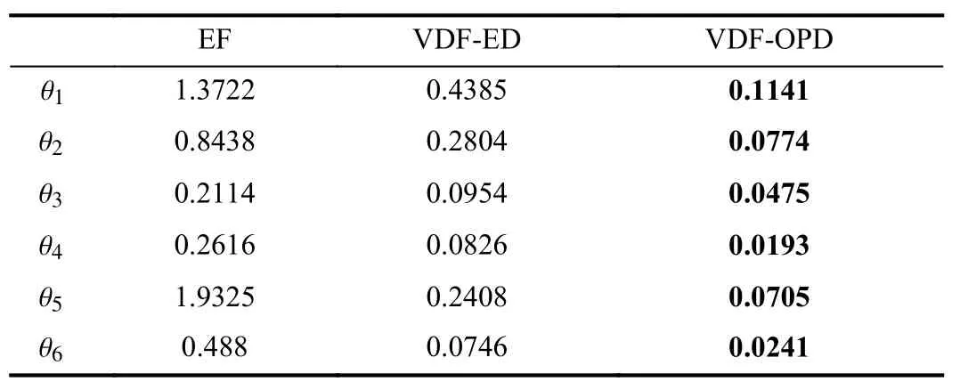
TABLE IRMSE OF PARAMETER ESTIMATES FROM EF,VDF-ED,AND VDF-OPD ALGORITHMS
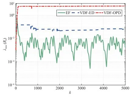
Fig.3.λ min(Rk) in EF,VDF-ED,and VDF-OPD algorithms.
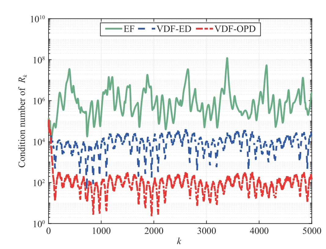
Fig.4.Condition number of Rk in EF,VDF-ED,and VDF-OPD algorithms.
VII.CONCLUSIONS
In this paper,a new VDF algorithm using oblique projection decomposition is presented for MO systems under nonpersistent excitation.It ensures the information matrix is lower and upper bounded,and its estimation error variance converges.In contrast,the VDF-ED algorithm in [23]discounts old information in part of its forgotten subspace where no new information is received,hence producing a more ill-conditioned information matrix under non-persistent excitation.The advantage of our proposed algorithm is illustrated by a numerical simulation example.
APPENDIX A
PRELIMINARIES ON OBLIQUE PROJECTIONAPPENDIX B
Let X and Y be complementary subspaces of Rn,i.e.,X +Y=RnandX∩Y={0}.Note that Xand Yarenot necessarily orthogonal.The oblique projector onto X alongY is uniquely represented by a square matrixPX|Y∈Rn×nthat satisfies
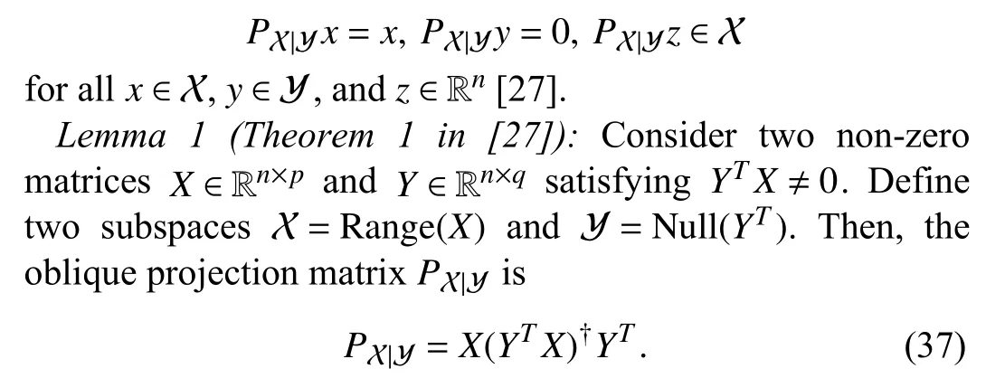
If X+Y=Rnand X∩Y={0},the two oblique projectionsPX|YandPY|Xare complementary,i.e.,PX|Y+PY|X=In.
Note that the oblique projection matrixPX|Yin (37) is idempotent but can be non-symmetric.If X and Y in Lemma 1 are orthogonal complementary subspaces,PX|Ybecomes an idempotent and symmetric matrix representing the orthogonal projection onto X.
PROOF OF THEOREM 1
APPENDIX C
PROOF OF THEOREM 2APPENDIX D
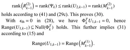
With the two complementary subspaces Vk-1in (16) andin(15),the applied oblique projection in (12)results in

due toRk-1>0 and (26).Note that (26) can be expressed as,withcolidenotingtheithcolumn of amatrix.Accordingto (25)withϵth=0,if coli(Ψk)is nonzero,the associated coli(Uk-1) should be included in the forgotten part,i.e.,U2,k-1in (27).Otherwise,coli(Uk-1) is included in the retained part,i.e.,U1,k-1in (27).Hence rank(U2,k-1)is equal to the number of non-zero columns of Ψk.Furthermore,since rank(Ψk) is less than or equal to the number of non-zero columns of Ψk,we have rank(Ψk)≤rank(U2,k-1),thus
PROOF OF THEOREM 3
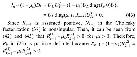
In the following,we prove thatRkobtained from (23) is positive ifRk-1is positive and Φkis bounded.This then leads to the proof of Theorem 3 via mathematical induction.
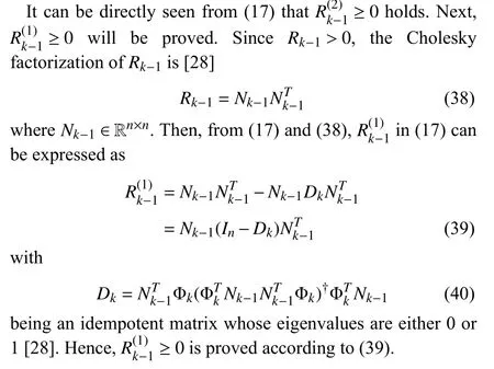
From (17) and (38)–(40),we have

SinceDkis an idempotent matrix,its eigenvalue decomposition can be expressed as

withs=rank(Dk).Then,we have
APPENDIX E
PROOF OF THEOREM 4
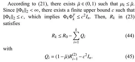
Assume rank(Φk)=rk,whererkmay vary with Φk.Let the singular value decomposition of Φkbe expressed as
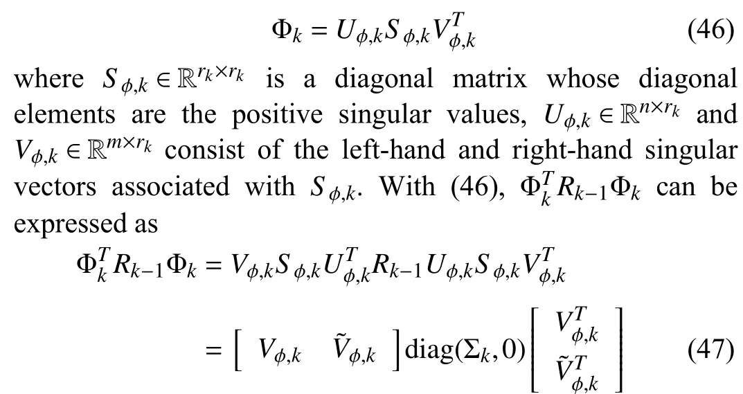
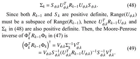

From (46) and (50),Qiin (45) can be expressed as

Then,using the invariance property of trace under cyclic permutations,the trace ofQican be rewritten as


Let λi-1,jrepresent thejth eigenvalue ofRi-1.Then,thejth eigenvalue of Ωi-1in (52) is

Next,by following the same idea in the proof of Theorem 2 in [21],we prove that it is impossible to have an unboundedRkby contradiction.Assume that one eigenvalueλi-1,s(1 ≤s≤n) ofRi-1is unbounded.Then,at all time instantsq≥i,the eigenvalue λq,sofRqbecomes unbounded according to the update ofRqin (23) fromRq-1.Hence,for allq≥i,the eigenvalue ωq,sin (54) is unbounded.Furthermore,each tr(Qi)in (52) is dominated by the ratio

th(at is unbound)ed.Therefore,on the right-hand side of (44),becomes negative and unbounded,which is in contradiction with the positive definiteness ofRkproved in Theorem 3.Such a contradiction proves thatRkmust be bounded from above.
APPENDIX F
PROOF OF THEOREM 5

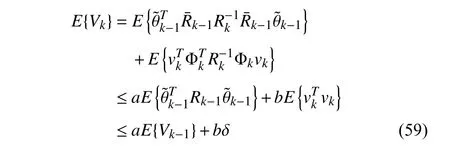
Under the condition ‖Φk‖2>ε,holds due to the adopted forgetting strategy.Hence there existsa∈(0,1) such that (34) holds for allk>0.According to (56),there must also existb∈(0,1) such that (35) holds for allk≥0.
From (19),(20),(22),(32),and (33),the parameter estimation error dynamics is expressed as
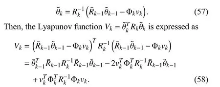
Taking mathematical expectation on both sides of (58),we haveE{Φkvk}=0 due to the statistical independence betweenvkand Φk,then we derive
杂志排行
IEEE/CAA Journal of Automatica Sinica的其它文章
- Deep Learning Based Attack Detection for Cyber-Physical System Cybersecurity: A Survey
- Sliding Mode Control in Power Converters and Drives: A Review
- Cyber Security Intrusion Detection for Agriculture 4.0: Machine Learning-Based Solutions,Datasets,and Future Directions
- Barrier-Certified Learning-Enabled Safe Control Design for Systems Operating in Uncertain Environments
- Cubature Kalman Filter Under Minimum Error Entropy With Fiducial Points for INS/GPS Integration
- Conflict-Aware Safe Reinforcement Learning:A Meta-Cognitive Learning Framework
