A PID-incorporated Latent Factorization of Tensors Approach to Dynamically Weighted Directed Network Analysis
2022-01-26HaoWuXinLuoMengChuZhouMuhyaddinRawaKhaledSedraouiandAiiadAlbeshri
Hao Wu,Xin Luo,,MengChu Zhou,,Muhyaddin J.Rawa,,Khaled Sedraoui,and Aiiad Albeshri
Abstract—A large-scale dynamically weighted directed network(DWDN) involving numerous entities and massive dynamic interaction is an essential data source in many big-data-related applications,like in a terminal interaction pattern analysis system(TIPAS).It can be represented by a high-dimensional and incomplete (HDI) tensor whose entries are mostly unknown.Yet such an HDI tensor contains a wealth knowledge regarding various desired patterns like potential links in a DWDN.A latent factorization-of-tensors (LFT) model proves to be highly efficient in extracting such knowledge from an HDI tensor,which is commonly achieved via a stochastic gradient descent (SGD)solver.However,an SGD-based LFT model suffers from slow convergence that impairs its efficiency on large-scale DWDNs.To address this issue,this work proposes a proportional-integralderivative (PID)-incorporated LFT model.It constructs an adjusted instance error based on the PID control principle,and then substitutes it into an SGD solver to improve the convergence rate.Empirical studies on two DWDNs generated by a real TIPAS show that compared with state-of-the-art models,the proposed model achieves significant efficiency gain as well as highly competitive prediction accuracy when handling the task of missing link prediction for a given DWDN.
I.INTRODUCTION
IN this era of big data,a large-scale dynamically weighted directed network (DWDN) representing dynamic interactions among massive entities is frequently encountered in various big data analysis projects [1]–[5].Its examples include a terminal interaction network [6],[7],a social network [8],[9],and a wireless sensor network [10],[11].However,owing to the huge number of involved entities,it becomes impossible to observe their full interactions,making a corresponding DWDN high-dimensional and incomplete(HDI).For instance,a terminal interaction pattern analysis system (TIPAS) concerned in this study focuses on a largescale terminal interaction network that involves 1 400 742 terminals (e.g.,personal computers,intellectual mobiles and servers) and 77 441 650 directed interactions scattering in 1158 time slots.Its dimensions come to 1 400 742 × 1 400 742 ×1158,while its data density (known data entry count over total) is about 3.41 × 10⁻⁸only.Despite its HDI nature,it contains rich knowledge describing various desired patterns like potential links and abnormal terminals [1],[2].Therefore,determining how to acquire such desired knowledge from it becomes a thorny issue.
To date,researchers have proposed a myriad of data analysis models for extracting useful knowledge from an unweighted network.For example,a static network can be analyzed through a node similarity-based model [12],a metropolis-hasting random walk model [13],a kernel extreme learning machine-based model [14],and a random walk-based deepwalk model [15].When a target network is dynamic,its knowledge acquisition can be implemented through a kernel similarity-based model [16],a Louvain-based dynamic community detection model [17],a spectral graph wavelet model [18],and a dynamic node embedding model [19].The above mentioned models are able to perform knowledge discovery given an unweighted network.However,they are incompatible with DWDN with directed and weighted links.
On the other hand,an HDI tensor is able to fully preserve a DWDN’s structural,spatial and temporal patterns [20],[21],making it possess inherent advantages in describing DWDN.Therefore,a latent factorization-of-tensors (LFT)-based approach to DWDN representation learning has become popular in recent years [22]–[26].Representative models of this kind include a regularized tensor decomposition model[22],a Candecomp/Parafac (CP) weighted optimization model[23],a biased non-negative LFT model [24],a fused CP factorization model [25],and a non-negative CP factorization model [26].
When building an LFT-based model,stochastic gradient descent (SGD) is mostly adopted as the learning algorithm to build desired latent features (LFs) [27]–[29].However,an SGD-based LFT model updates an LF depending on the stochastic gradient defined on the instant loss only,without considering historical update information.Consequently,it takes many iterations to convergence,thus resulting in low computational efficiency given large-scale DWDNs from industrial applications [30]–[32].For instance,considering the aforementioned DWDN generated by a real TIAPS,an SGDbased LFT model needs to traverse 77441650 entries in one iteration,which is computationally expensive.
A proportional-integral-derivative (PID) controller utilizes the past,current and future information of prediction error to control an automated system [33],[34].It has been widely adopted in various control-related applications [35],[36],e.g.,a digital fractional order PID controller for a magnetic levitation system [37],a PID passivity-based controller for the regulation of port-Hamiltonian systems [38],a cascaded PID controller for automatic generation control analysis [39],and a nonlinear self-tuning PID controller for position control of a flexible manipulator [40].However,a PID-based method is rarely adopted in HDI tensor representation,which is frequently encountered in many big data-related applications[31],[32].
Motivated by the above discovery,the following research question is proposed:
Research Question:Is it possible to incorporate the PID principle into an SGD-based LFT model,thereby improving its performance on an HDI tensor?
To answer it,this work innovatively proposes a PIDincorporated LFT (PLFT) model,which seamlessly integrates the PID control principle into an SGD solver.A PLFT model’s main idea is to construct an adjusted instance error by using a PID controller,and then adopt this adjusted error to perform an SGD-based learning process,thereby improving the convergence rate.This work aims to make the following contributions:
1) A PLFT model.It performs latent feature analysis on an HDI tensor with high efficiency and preciseness;
2) Detailed algorithm design and analysis for PLFT.It provides specific guidance for researchers to implement PLFT for analyzing DWDNs.
Empirical studies on two large-scale DWDNs from a real TIPAS demonstrate that compared with state-of-the-art models,PLFT achieves impressively high efficiency as well as highly competitive prediction accuracy for link prediction.
The remainder of this paper is organized as follows.Section II provides the preliminaries.Section III provides a detailed description of PLFT.Section IV reports experimental results.Section V discusses related work.Finally,Section VI concludes this paper.
II.PRELIMINARIES
A.Symbols Appointment
Adopted symbols in this paper are summarized in Table I.
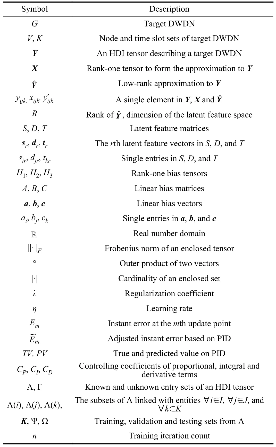
TABLE IADOPTED SYMBOLS AND THEIR DESCRIPTIONS
B.A DWDN and an HDI Tensor
Fig.1 depicts a small example illustrating the connections between a DWDN and an HDI tensor.Consider the dynamic states of a DWDN during |K| time slots.The net can be described by a snapshot sequence where each one describes its state observed during a specified time slot.
Definition 1 (DWDN State):Gk= (V,Lk) is thekth state of a DWDN whereLkis the weighted directed link set observed at time slotk∈K= {1,2,...,|K|}.
An HDI tensor can accurately describe a DWDN [24],[25].Formally,it is defined as follows.
Definition 2 (HDI Tensor):Given entity setsI,J,andK,letY|I|×|J|×|K|∈ R be a tensor where each entryyijkrepresents certain relationship among entitiesi∈I,j∈Jandk∈K.GivenY’s known and unknown entry sets Λ and Γ,Yis an HDI tensor if |Λ| ≪ |Γ|.
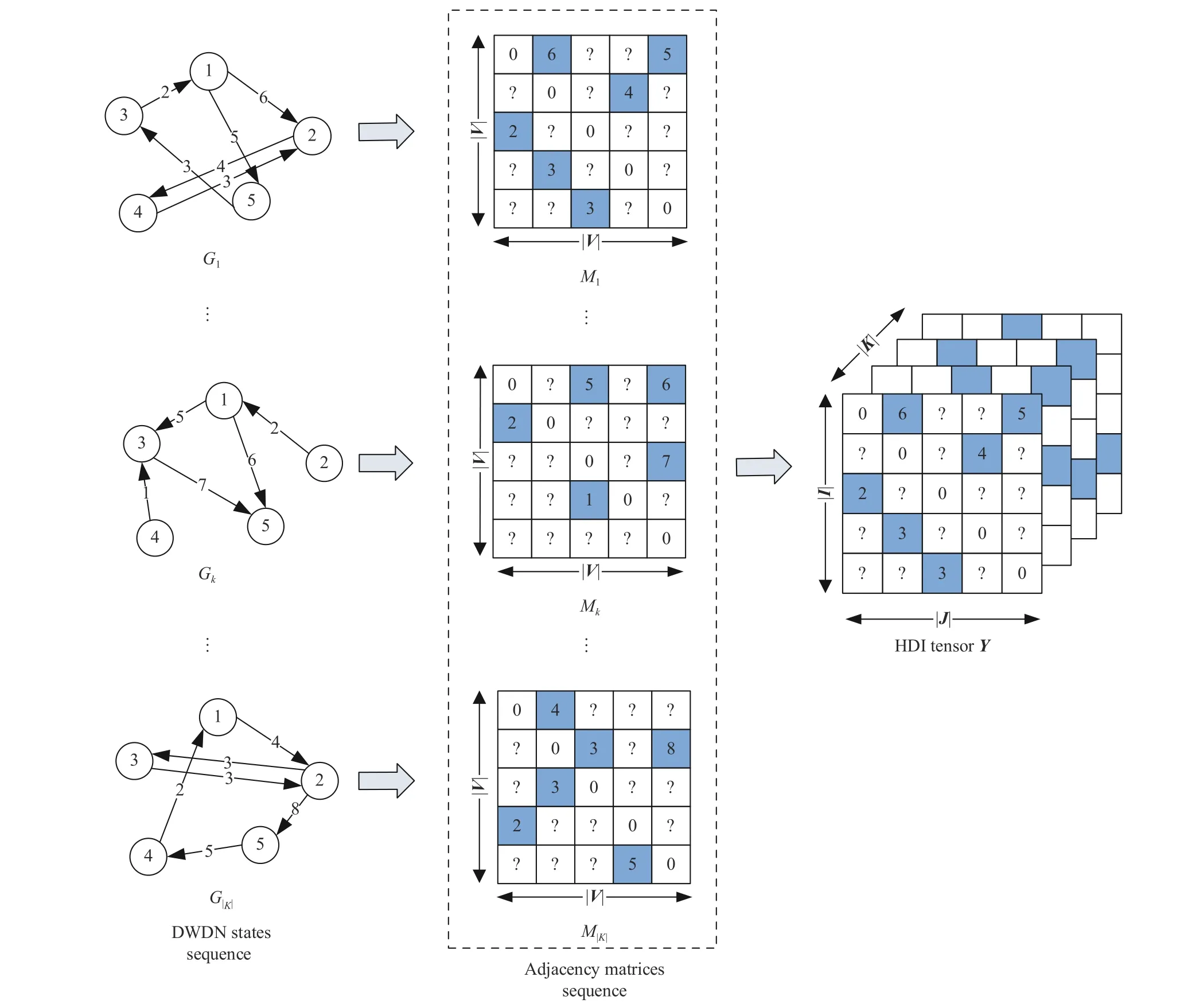
Fig.1.A DWDN and an HDI tensor Y.
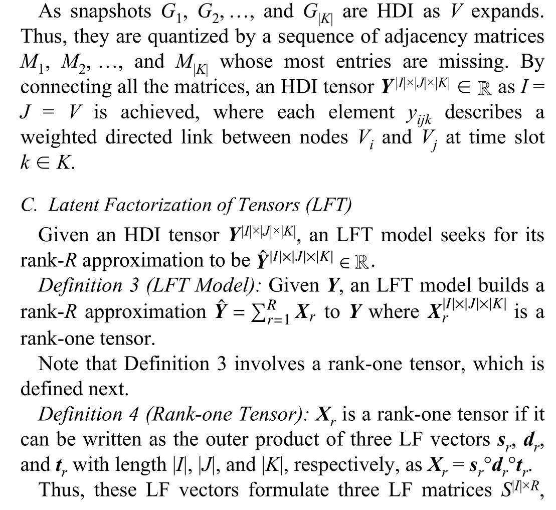
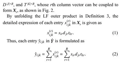
To obtain three LF matricesS,DandT,we build an objective functionεto measure the difference betweenYand,which relies on the commonly-used Euclidean distance[21]–[25]

As shown in Fig.2,Yis an HDI tensor with only a few known entries.Hence,we defineεon Λ only to representY’s known entries precisely [20],[24],[28],[29] to reformulate(3) as
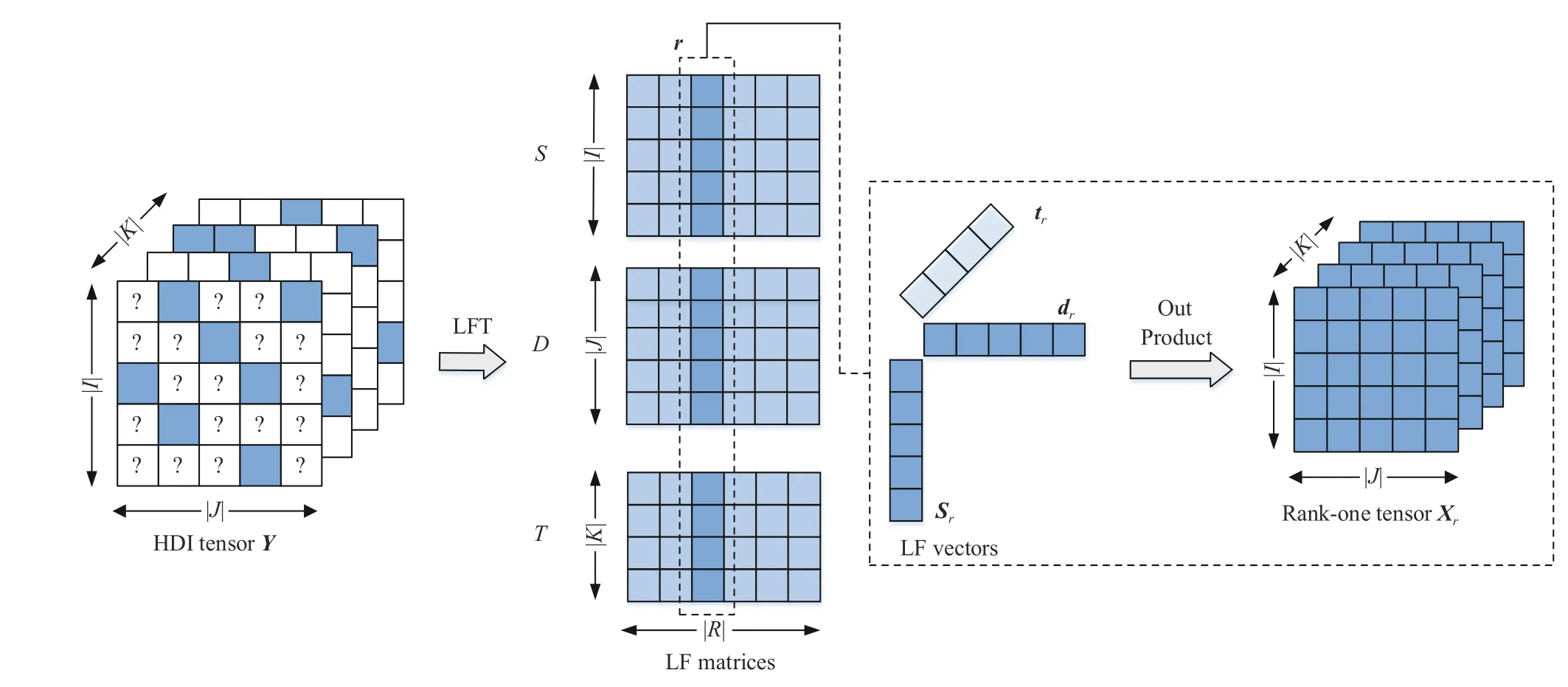
Fig.2.Latent factorization of an HDI tensor Y.

According to prior research [24]–[26],due to the imbalanced distribution ofY’s known entries,it is essential to incorporate Tikhonov regularization into (4) to avoid overfitting

With SGD,the learning scheme for desired LFs is given as
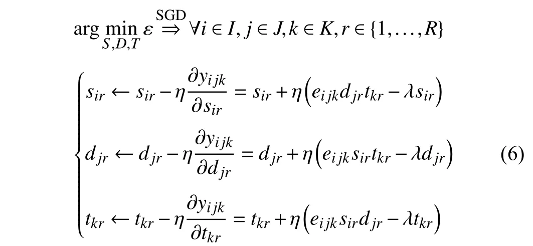
whereeijk=denotes the instant error onyijk.With (6),an SGD-based LFT model can extract latent patterns form an HDI tensor.For instance,Fig.3 depicts the process of performing missing link prediction forGthrough an LFT model.
D.A PID Controller
A PID controller adjusts the observed error based on proportional,integral,and derivative terms [33]–[36].Fig.4 depicts the flowchart of a discrete PID controller.Note that this paper adopts this base controller because it is directly compatible with an SGD-based LFT model’s learning scheme as shown later.As shown in Fig.4,at themth time point,a discrete PID controller builds the adjusted erroras follows:

whereEmandEiare the observed error at themandith time points,CP,CIandCDare the coefficients for controlling the proportional,integral and derivative effects,respectively.With the adjusted error,the system considers prior errors to implement precise control.Next,we integrate the PID control principle into SGD-based LFT to achieve a PLFT model.
III.PLFT MODEL
A.Model
According to [41]–[43],an LFT model’s stability and representation learning ability can be enhanced by incorporating linear bias (LB) into its learning objective.According to [24],for a three-way HDI tensorY|I|×|J|×|K|,the LBs can be modeled through three LB vectorsa,b,andcwith length |I|,|J|,and |K|.By introducing them into (5),we arrive at the biased learning objective given as

With (8),consists ofRrank-one tensors {Xr|r∈ {1,…,R}} built on LF matricesS,DandT,and three rank-one bias tensorsH1–H3built on LB matricesA,BandC.The LB vectorsa,bandcare respectively set as the first,second and third columns ofA,BandC,and other columns are set as onevalued column vectors,which is similar to LBs involved in a matrix factorization model [42],[43].This design is shown in Fig.5.
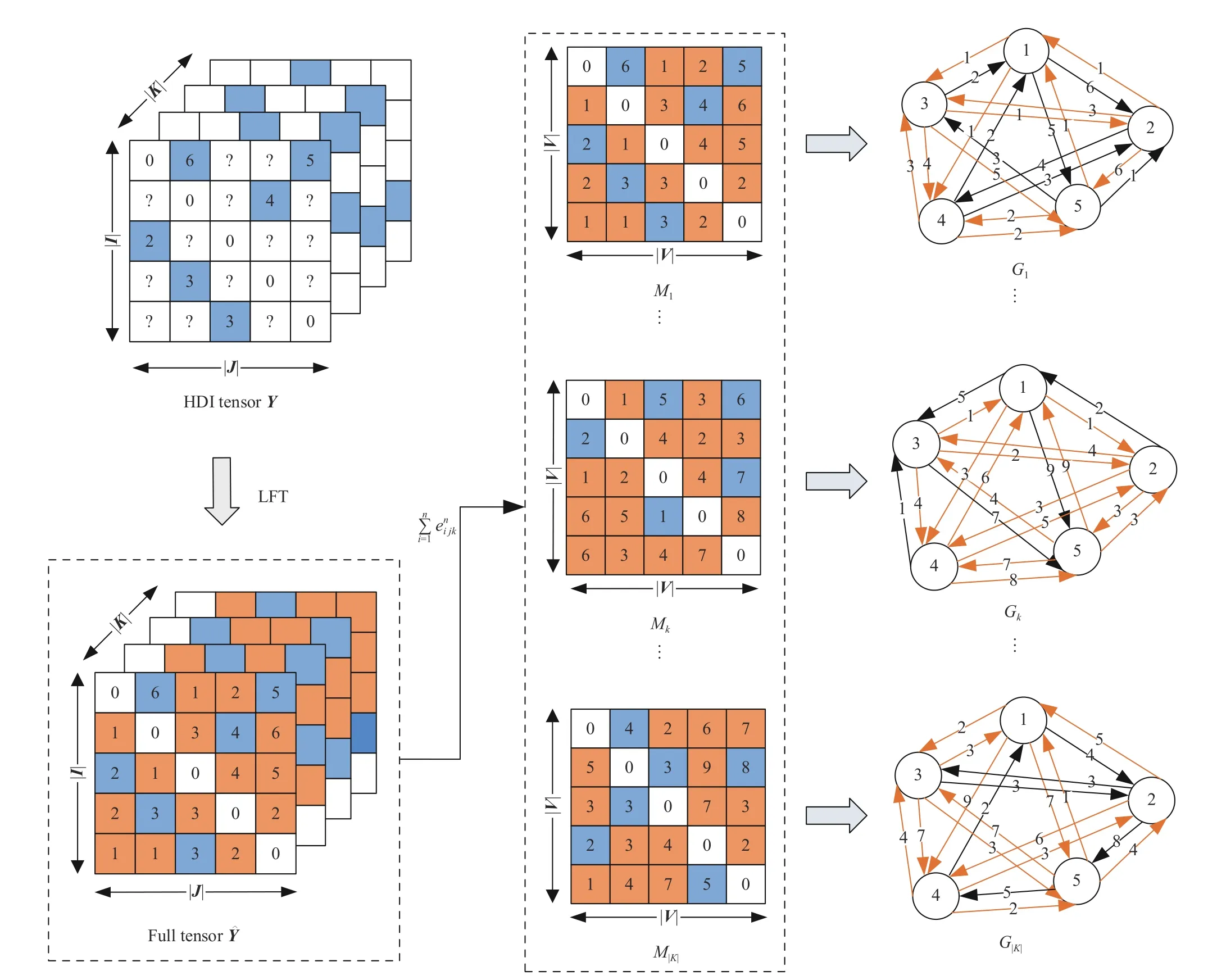
Fig.3.Missing link prediction by performing LFT on an HDI tensor Y.
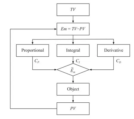
Fig.4.Flow chart of a discrete PID controller.
As given in (5),with SGD,the instant error of an instanceyijkat thenth training iteration is.Following(7),such instant error can be regarded as a PID controller’s proportional term.Moreover,the information ofyijkis passed into a parameter update througheijkonly in a training iteration.Therefore,this process can be described by a simplified PID controller by settingCP= 1 andCI=CD= 0.
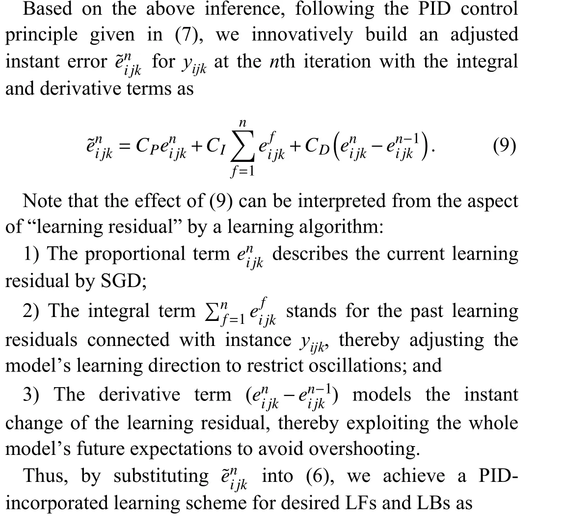
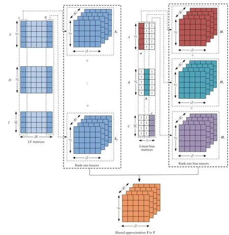
Fig.5.Building HDI tensor Y’s biased approximation tensor .
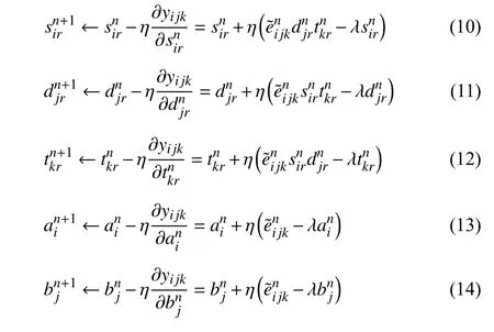

With (10)–(15) a PLFT model is achieved.Its flow is in Fig.6.
B.Algorithm Design and Analysis
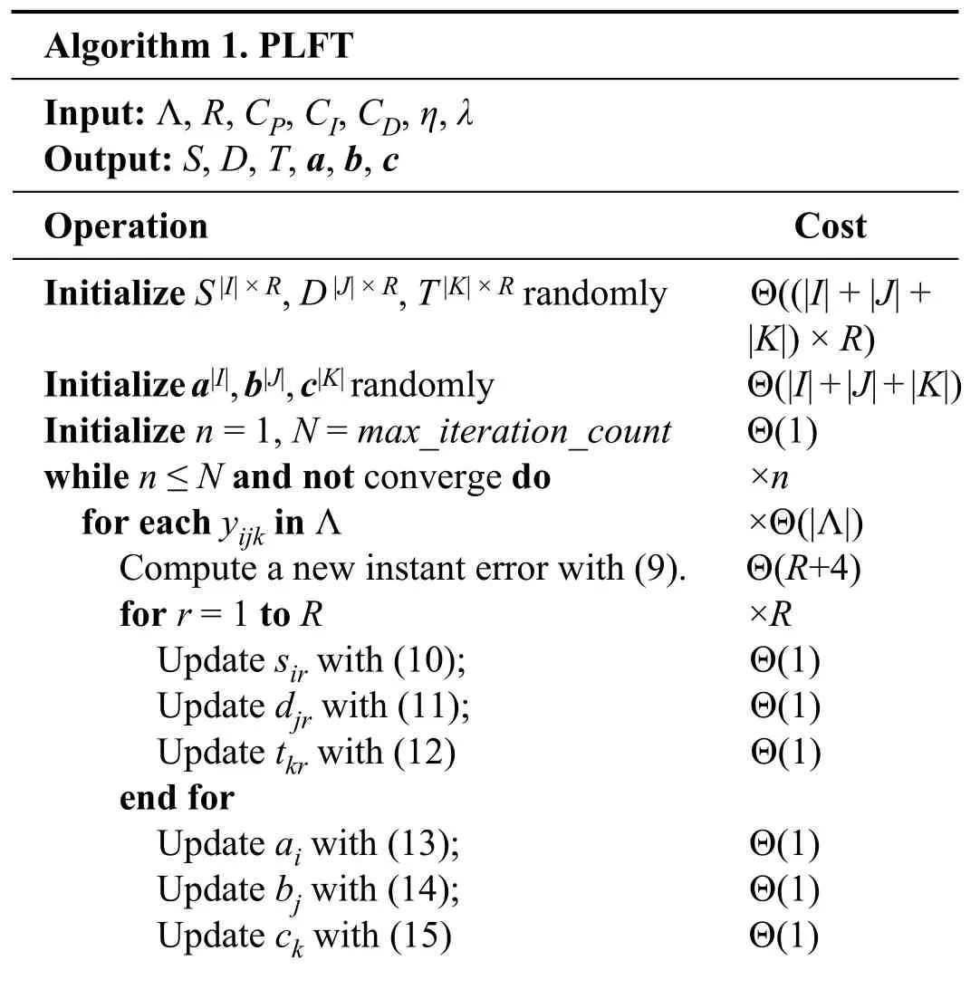
Based on the above inferences,we design Algorithm PLFT.According to PLFT,the main task in each iteration is to update LF matrices and LB vectors.Hence,its computation cost is

Note that (16) adopts the condition that |Λ| ≫ max{|I|,|J|,|K|} which is constantly fulfilled in real applications.SincenandRare positive constants in practice,a PLFT model’s computation cost is linear with an HDI tensor’s known entry count.
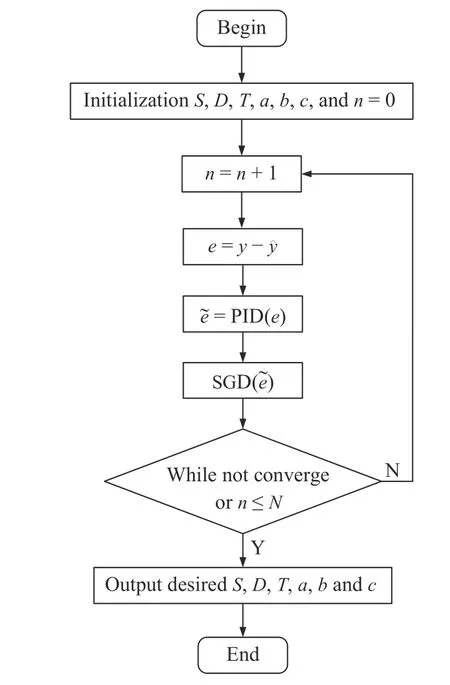
Fig.6.Flowchart of PLFT.
Its storage cost mainly depends on the following three factors: 1) arrays caching the input known entries Λ and the corresponding estimations; 2) auxiliary arrays caching the integral and derivative terms on each instance; and 3) LF matricesS,DandT,and linear vectorsa,bandc.Hence,the PLFT’s storage cost is given as

which is linear with the target HDI tensor’s known entry count and its LF count.The next section conducts experiments to validate a PLFT model’s performance.
IV.EXPERIMENTAL RESULTS AND ANALYSES
A.General Settings
Datasets:The experiments are conducted on two large-scale DWDNs labeled asD1 andD2 from a real TIPAS that concerns the dynamic interactions over two million terminals.Table II summarizes their details.On them,we build two different HDI tensors,e.g.,the HDI tensor corresponding toD1 has the size of 1 400 742 × 1 400 742 × 1158 and data density of 8.41 × 10⁻⁸only.

TABLE IIDATASET DETAILS
To achieve objective results,each dataset is randomly split into the disjoint training setK,validation set Ψ,and testing set Ω at the ratio of 7:1:2.A tested model is built onK,validated on Ψ,and tested on Ω to obtain the final outcomes.The training process of a model terminates if 1) the number of consumed iterations reaches a preset threshold,e.g.,500,or 2)it converges,i.e.,the error difference between two consecutive iterations is less than 10–6.Note that for all involved models,the LF space dimensionRis fixed at 20 uniformly to balance their computational cost and representation learning ability,following the settings in [20]–[25].
Evaluation Metrics:We choose weighted missing link prediction as the evaluation protocol due to the great need of building full interaction mapping among involved entities in real systems [20]–[25].The root mean squared error (RMSE)and mean absolute error (MAE) are the evaluation metrics
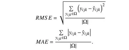
Note that for a tested model,a small RMSE and MAE denote high prediction accuracy for missing links in a DWDN.
B.Parameters Sensitivity Test
As shown in Section III,PLFT’s performance is affected by learning rateη,regularization coefficientλ,and PID constantsCP,CI,andCD.Thus,we start with parameter sensitivity tests.
1) Effects of η and λ
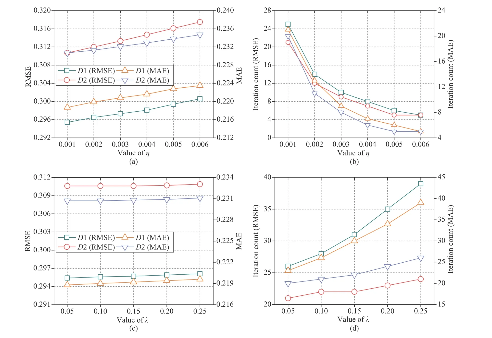
Fig.7.Impacts of η and λ.
This set of experiments fixes the PID coefficients and makesηincrease from 0.001 to 0.006 andλfrom 0.05 to 0.25.Figs.7(a) and 7(c) records PLFT’s RMSE and MAE asηand λ changes.Figs.7(b) and 7(d) depicts the corresponding iteration count.From these results,we have the following findings:
a) PLFT’s convergence is related with η and λ:As shown in Figs.7(b) and 7(d),the converging iteration counts of PLFT in RMSE and MAE decrease asηincreases while they increase asλincreases onD1 andD2.For instance,as shown in Fig.7(b),asηincreases from 0.001 to 0.006 onD2,the converging iteration count of PLFT decreases from 21 to 5 in RMSE,and from 20 to 5 in MAE,respectively.This results is consistent with the role ofηin PLFT,i.e.,the larger the learning rate,the faster the parameter update velocity,resulting in fewer iterations for convergence.However,we also note that owing to its incorporation of PID,PLFT’s convergence rate stays consistently high even if the learning rate is set to be small.On the other hand,as shown in Fig.7(d),PLFT’s converging iteration count is generally linear withλ.For instance,asλincreases from 0.05 to 0.25 onD2,its converging iteration count increases from 21 to 24 in RMSE,and from 20 to 26 in MAE.This is because whenλgrows larger,the parameter update process requires more fitting regularization term,which leads to more iterations.
b) PLFT’s prediction error increases as η and λ increase:For instance,as depicted in Fig.7(a),PLFT’s RMSE is 0.2954 and 0.3004 asη= 0.001 and 0.006 onD1,where the increment ((RMSEhigh–RMSElow)/RMSEhigh) is 1.66%.This result indicates that sinceηgrows larger,the parameter update process overshoots an optimum.As shown in Fig.7(c),PLFT’s RMSE is 0.2954 and 0.2961 asλincreases from 0.05 to 0.25 onD1,where the increment is 0.24%.This phenomenon demonstrates the occurrence of underfitting asλincreases continually.Note that similar situations are seen onD2,as shown in Figs.7(a) and 7(c).In general,the PLFT’s prediction error increases more rapidly inηthan inλ.
2) Effects of CP,CI,andCD
This set of experiments fixesηandλ,and makes the PID coefficients increase to test their effects on PLFT’s performance.The experimental results are illustrated in Fig.8.From them,we have the following findings:
a) PLFT’s converging iteration count relies on CP,CI,and CD:As shown in Figs.8(b) and 8(d),PLFT’s converging iteration count in RMSE and MAE decreases asCPandCIincrease.However,it increases asCDincreases as shown in Fig.8(f).For instance,as shown in Fig.8(b),onD1,PLFT’s converging iteration count in RMSE is 57 withCP= 1.WhenCPincreases to 5,it decreases to 23.Likewise,asCIincreases from 0.01 to 0.09,it decreases from 34 to 15.In contrast,PLFT’s converging iteration count in RMSE increases from 24 to 43 asCDincreases from 10 to 90.Similar phenomena are encountered onD2 as shown in Figs.8(b),8(d) and 8(f).
b) CP and CI affect PLFT’s prediction error slightly:As shown in Fig.8(a) and 8(c),onD1 andD2,PLFT’s RMSE and MAE increase slightly withCPandCI,while they are generally steady asCDincreases.For instance,onD1,as shown in Fig.8(a),PLFT’s MAE increases from 0.2180 to 0.2196 asCPincreases from 1 to 5,where the increment is 0.73%.According to Fig.8(c),PLFT’s MAE is 0.2184 withCI= 0.01 and 0.2193 withCI= 0.09,where the increment is 0.42%.In comparison,as shown in Fig.8(e),whenCDincreases from 10 to 90,the difference in PLFT’s MAE is 0.0002 only.Similar results are obtained onD2,as shown in Figs.8(a),8(c) and 8(e).
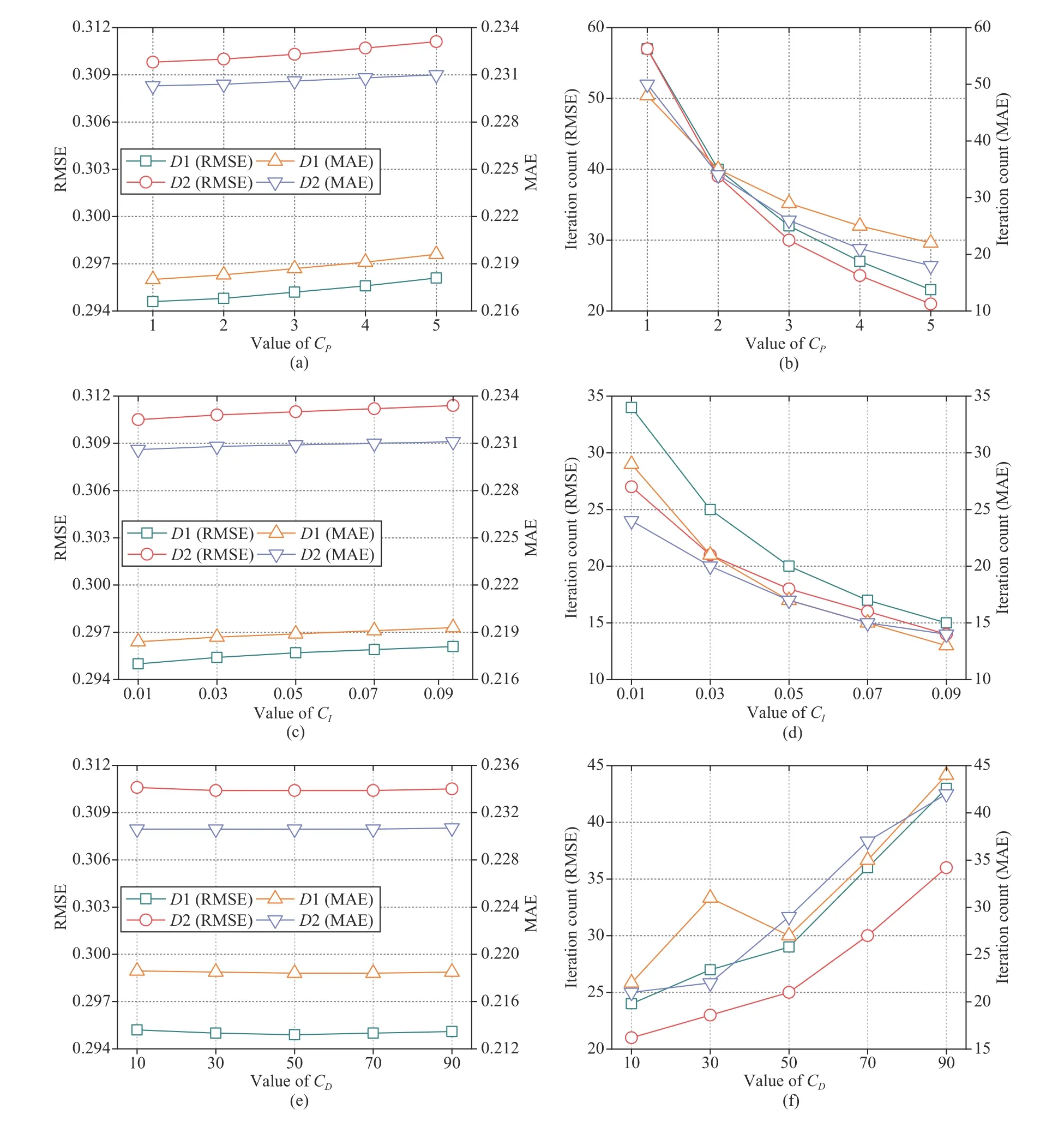
Fig.8.Impacts of CP,CI and CD.
Note that the above results are consistent with the theoretical analysis in Section III-A.CPcontrols the proportional term,and actually plays the role of the learning rate in the current update.CIcontrols the adjustment of a learning direction.Accordingly,a largerCIhas a stronger restriction on the oscillation of a parameter update process,which can make PLFT converge faster but also cause slight accuracy loss.CDcontrols the future expectations of a parameter update process.CDin an appropriate range can effectively avoid overshooting.Moreover,a relatively smallCDcan make PLFT converge faster to an optimum.
3) Summary
Based on the above results,we summarize that PLFT’s convergence rate is sensitive in its hyper-parameters,while its prediction accuracy is less sensitive in them.However,to further increase a PLFT model’s practicability in addressing DWDN analysis problems,a hyper-parameter self-adaptive scheme is desired.We plan to address it as a future issue.
C.Comparison With State-of-the-art Models
Three state-of-the-art models with the ability of analyzing an HDI tensor are compared with the proposed model.Their details are as follows:
a) M1:A time-SVD++ model [44].It models the temporal effects into the objective function of a latent factor model such that the model can well represent an HDI tensor.

TABLE IIIHYPER-PARAMETERS SETTINGS OF M1-M4
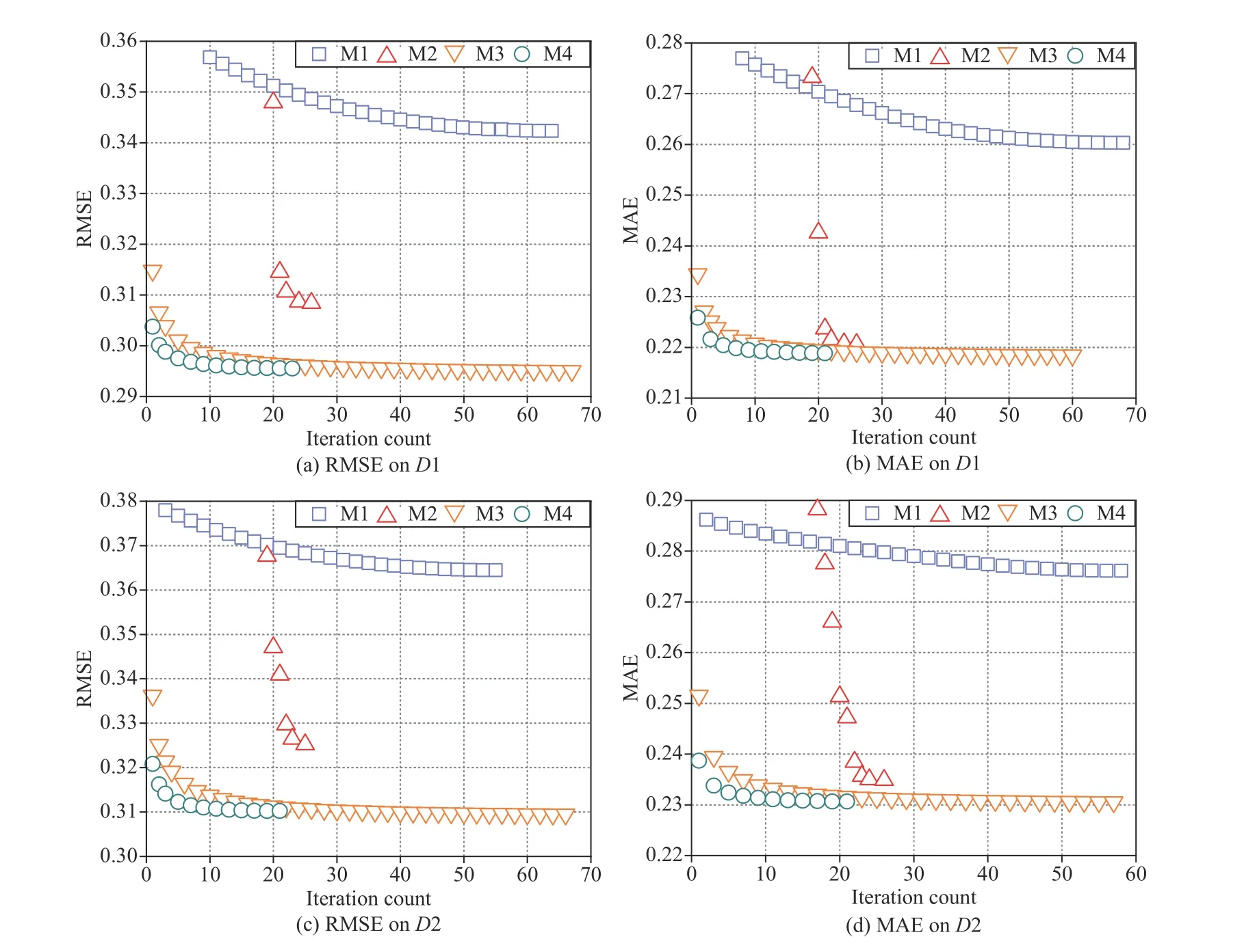
Fig.9.Training curves of M1–M4 on D1 and D2.
b) M2:A PARAFAC decomposition-based model [45].It builds anl1norm-based regularization scheme,and adopts nonnegative alternating least squares as its learning scheme.
c) M3:An SGD-based LFT model [29].It adopts a standard SGD to perform parameters learning.
d) M4:A PLFT model proposed in this paper.
Note that hyper-parameter settings of M1–M4 are given in Table III.Considering M1–M4,we perform a grid search for their related hyper-parameters on one set of experiments out of 20 independent runs in total to achieve their best performance,and then adopt the same settings on the remaining 19 sets of experiments.
Fig.9 depicts M1–M4’ training curves.Fig.10 records their total time costs.Fig.11 depicts their RMSE and MAE.From these results,we have the following important findings:
a) M4 converges much faster than its peers do:As shown in Fig.9(a),M4 takes 23 iterations only to converge in RMSE on D1.In comparison,M1–M3 takes 64,26 and 67 iterations to converge in RMSE onD1,respectively.Considering MAE,as shown in Fig.9(b),M1–M3 respectively requires 68,26 and 60 iterations to converge onD1,while M4 only consumes 21 iterations.Similar phenomena can be found onD2,as depicted in Figs.9(c) and 9(d).From these results,we can obviously see that by incorporating a PID control principle,PLFT’s convergence rate is improved significantly over an SGD-LFT model.It turns out that incorporating the PID control principle into an SGD-based LFT model is feasible and highly effective.
b) M4 achieves higher computational efficiency than its peers do:For instance,as shown in 10(a),onD1,M4 takes about 10 min to converge in RMSE,which is 8.13% of 123 min by M1,7.63% of 131 min by M2,and 40% of 25 min by M3.Considering MAE,M1 takes about 9 min to converge,which is 6.87% of 131 min by M1,6.62% of 136 min by M2,and 40.90% of 22 min by M3.Similar outputs are obtained onD2,as in Fig.10(b).As summarized in Algorithm 1,the computation cost of a PLFT model mainly relies on an HDI tensor’s known entry set.From the above experimental results,we evidently see that such design is extremely suitable and necessary when analyzing a large-scale HDI DWDN.
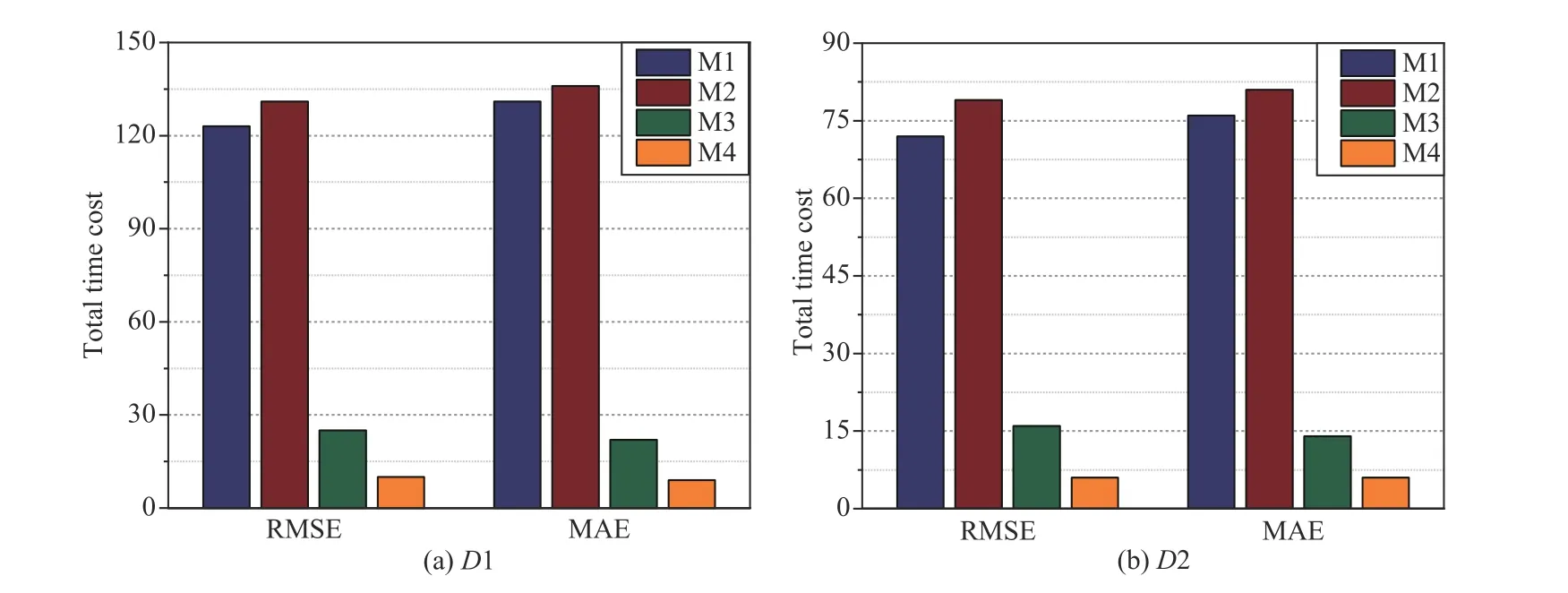
Fig.10.Total time cost (min) of M1–M4 on D1 and D2.
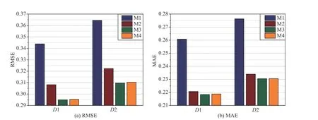
Fig.11.The RMSE and MAE of M1–M4 on D1 and D2.
c) M4 has highly competitive prediction accuracy for missing data of an HDI tensor when compared with its peers:As depicted in Fig.11(a),onD1,M4’s RMSE is 0.2954,which is about 14.10% lower than the 0.3439 RMSE obtained by M1 and 4.15% lower than the 0.3082 RMSE obtained by M2,but 0.14% higher than the 0.2950 RMSE obtained by M3.Likewise,onD2,M1–M4 respectively achieve RMSEs of 0.3645,0.3223,0.3096 and 0.3103,where the RMSE of M4 is 14.87% and 3.72% lower than that of M1 and M2 while 0.23% higher than that of M3.When measured by MAE,similar results are achieved on both datasets,as shown in Fig.11(b).Note that M4 suffers from a small accuracy loss when compared with M3.Yet its computational efficiency is much higher than that of M3.This phenomenon indicates the performance of a PLFT model can still be further improved by incorporating another advanced controller,e.g.,a nonlinear PID controller.We plan to address this issue in the next work.
D.Summary
According to the experimental results,we conclude that PLFT is equipped with: a) a high convergence rate,b)impressively high computational efficiency,and c) highly competitive prediction accuracy.Therefore,PLFT is a highly effective model to large-scale DWDNs analysis.
V.RELATED WORK
A network has become increasingly important to model a complex system consisting of numerous entities and interactions.Network data analysis is widely involved in many fields,where missing link prediction is one of the essential and vital tasks in network analysis [1]–[5].To date,many sophisticated models to missing link prediction in a given network are proposed.They can be roughly divided into the following three categories:
1)LF Analysis-based Models
Duanet al.[46] propose an ensemble approach,which decomposes traditional link prediction into sub-problems of smaller size and each sub-problem is solved with LF analysis models.Nguyenet al.[47] utilize LF kernels and cast the link prediction problem into a binary classification to implement link prediction on sparse graphs.Zhuet al.[48] propose a temporal latent space model for dynamic link prediction,where the dynamic link over time is predicted by a sequence of previous graph snapshots.Yeet al.[49] use nonnegative matrix tri-factorization to construct network latent topological features,which acquires the principal common factors of the network link structures.Wanget al.[50] present a fusion model to fuse an adjacent matrix and key topological metrics into a unified probability LF analysis-based model for link prediction,which considers both the symmetric and asymmetric metrics.
2)Neural Networks-based Models
Wanget al.[51] design a Bayesian-based relational network model that combines network structures and node attributes to predict missing links.Chenet al.[52] propose a dynamic link prediction model by combining long short-term memory and encoder-decoder mechanisms.Liet al.[53] develop a temporal-restricted Boltzmann machine-based deep network,which predicts missing links by utilizing individual transition variances and influence of local neighbors.Ozcanet al.[54]propose a multivariate link prediction model for evolving heterogeneous networks via a nonlinear autoregressive neural network.Liet al.[55] model the evolution pattern of each link in a network by incorporating a gradient boosting decision tree and temporal restricted Boltzmann machine.
3)Network Analysis-based Models
Groveret al.[56] map involved nodes into low-dimensional feature space and adopts a biased random walk method to implement link prediction.Fuet al.[57] utilize line graph indices along with original graph indices to implement link weight prediction.Wanget al.[58] develop a cold-start link prediction approach by establishing the connections between topological and non-topological information.Xiaet al.[59]design a model based on a random walk with restart,which can determine potential collaborators in academic social networks.Deet al.[60] design a novel framework by using a stacked two-level learning paradigm for link prediction,which integrates local,community,and global signals.
The above mentioned approaches can efficiently perform missing link prediction on a specified network.However,they all fail to address DWDN with directed and weighted missing links.Moreover,they commonly suffer from high computational cost due to their model structure or learning scheme.In comparison,the proposed PLFT model describe a DWDN via an HDI tensor smoothly,and achieves high efficiency via incorporating the PID principle into its learning scheme.
VI.CONCLUSIONS
In order to improve an SGD-based LFT model’s efficiency,this work proposes a PLFT model that combines the information of past,current and future updates into its parameters update following the PID control principle,which is never seen in existing studies to our best knowledge.It exhibits a higher convergence rate and greater computational efficiency than state-of-the-art methods,and very competitive accuracy in missing link prediction in comparison with them.Hence,it provides highly effective solutions for large-scale DWDN analysis.However,the following issues remain open:
1) The performance of a PLFT model is affected by its hyper-parameters.Thus,making them adaptable to various applications is of great importance [61],[62].
2) A nonlinear PID [40],[63] has shown excellent performance in real applications.Thus,we may consider further performance gain by incorporating its principle into an SGD-based LFT model.
3) Determining how to further improve PLFT’s computational efficiency via a parallel computation framework [64]–[65],and apply PLFT to other datasets [66]–[69].We plan to address them as our future work.
杂志排行
IEEE/CAA Journal of Automatica Sinica的其它文章
- Deep Learning Based Attack Detection for Cyber-Physical System Cybersecurity: A Survey
- Sliding Mode Control in Power Converters and Drives: A Review
- Cyber Security Intrusion Detection for Agriculture 4.0: Machine Learning-Based Solutions,Datasets,and Future Directions
- Barrier-Certified Learning-Enabled Safe Control Design for Systems Operating in Uncertain Environments
- Cubature Kalman Filter Under Minimum Error Entropy With Fiducial Points for INS/GPS Integration
- Conflict-Aware Safe Reinforcement Learning:A Meta-Cognitive Learning Framework
