The Simulation of Five Tropical Cyclones by Sample Optimization of Ensemble Forecasting Based on the Observed Track and Intensity

Jihang LI ,Zhiyan ZHANG ,Lu LIU ,Xubin ZHANG* ,Jingxuan QU ,and Qilin WAN

1Guangzhou Institute of Tropical and Marine Meteorology,Guangzhou 510640,China

2State Key Laboratory of Severe Weather,Chinese Academy of Meteorological Sciences,Beijing 100081,China

ABSTRACT The quality of ensemble forecasting is seriously affected by sample quality.In this study,the distributions of ensemble members based on the observed track and intensity of tropical cyclones (TCs) were optimized and their influence on the simulation results was analyzed.Simulated and observed tracks and intensities of TCs were compared and these two indicators were combined and weighted to score the sample.Samples with higher scores were retained and samples with lower scores were eliminated to improve the overall quality of the ensemble forecast.For each sample,the track score and intensity score were added as the final score of the sample with weight proportions of 10 to 0,9 to 1,8 to 2,7 to 3,6 to 4,5 to 5.These were named as“tr”,“91”,“82”,“73”,“64”,and“55”,respectively.The WRF model was used to simulate five tropical cyclones in the northwestern Pacific to test the ability of this scheme to improve the forecast track and intensity of these cyclones.The results show that the sample optimization effectively reduced the track and intensity error,“55”usually had better performance on the short-term intensity prediction,and“tr”had better performance in short-term track prediction.From the overall performance of the track and intensity simulation,“91”was the best and most stable among all sample optimization schemes.These results may provide some guidance for optimizing operational ensemble forecasting of TCs.

Key words:tropical cyclones,ensemble forecast,sample optimization,observed track and intensity

1.Introduction

Ensemble forecasting is widely used in numerical weather prediction (Richardson,2000;Palmer,2002;Saetra et al.,2004;Cloke and Pappenberger,2009;Bougeault et al.,2010;Dupont et al.,2011;Fortin et al.,2014;Taillardat et al.,2016;Li et al.,2018a,2020a).However,in most cases,some of the ensemble samples do not reflect the observed outcomes,and these outliers can reduce the accuracy of the ensemble forecast.Fortunately,sample optimization is a good way to help resolve this problem (Saetra et al.,2004;Li et al.,2018b).

It is generally known that tropical cyclones (TCs) usually cause serious damage (Rappaport,2014;Torn,2016;Colby,2019).The reduction in TC track forecast errors is very dramatic in just 25 years due to global modeling advances,improvements in data assimilation,dramatic increases in observations primarily derived from satellite platforms,and use of ensemble forecast techniques (Landsea and Cangialosi,2018).Substantial efforts in recent years have focused on extracting additional information from ensembles.This type of research seeks to improve ensemble mean forecasts by selecting or weighting individual members by their performance at short lead times,near the time that the forecasts become available (Qi et al.,2014;Dong and Zhang,2016).According to Kowaleski and Evans(2020),TC ensemble track forecasts from 153 initialization times during 2017–18 were clustered using regression mixture models.For five-cluster partitions,a pruning threshold of 10% affected 49% and 35% of ensembles,improving 69%–74% of the forecasts that were subjected to pruning.The above studies achieved good results in track prediction of TCs,but the intensity prediction has been ignored.Zhang(2018) determined the optimal-member forecasts according to the closeness of the perturbed ensemble members’ forecasts to the latest observations for both track and intensity.In Zhang (2018),the optimal-member forecasts were illustrated to be effective in improving TC precipitation and wind forecasting.Although great progress in forecast skill has been made in predicting the track of TCs,TC intensity forecasting remains a significant challenge in this regard.

Li et al.(2018b) developed a scheme for the sample optimization of an ensemble forecast.The results have been applied to simulate TCs,and good results have been achieved in track simulation.When using the WRF model to simulate 11 TCs (Li et al.,2020b),sample optimization of the ensemble forecast based on the observed track had a significant effect on improving the track prediction of TCs,but the intensity simulation showed only a slight improvement.Moreover,based only on the observed intensity,the simulation of the intensity was improved by sample optimization to some extent,but the track prediction became worse(Li et al.,2021).

Track and intensity have been considered to be important indicators for quantitative risk assessment and early coastal evacuation decisions (Hamill et al.,2011).Therefore,both track and intensity are very important to TC prediction.To improve the TC prediction,the standard of sample optimization should consider both the observed track and intensity of TCs at the same time.The main purpose of the present research is to explore what proportions of the observed intensity and track can obtain a better track and intensity forecast of TCs at the same time.The remainder of this paper is organized as follows.Section 2 describes the WRF model and the experimental design.The changes in 6-h cycles among different schemes are presented in Section 3.Section 4 presents the experimental results.The primary findings are summarized in the last section.

2.Methodology

2.1.Methodology of sample optimization

In this research,steps were included for sample optimization of ensemble forecasting and are described in this section.Here,a sample indicates one ensemble member.

First,samples were scored and ranked.Each ensemble had 60 samples.After the samples and observations were obtained,the track forecast error and intensity forecast error of each sample were calculated,respectively.The track forecast error is defined as the great-circle distance between the predicted position and the observed position of a TC taken at the same time.The intensity forecast error is the absolute error between the predicted minimum sea level pressure(MSLP) and the observed MSLP.For both track score and intensity score at the same hour,the sample with the smallest error ranked first and had the highest score (60);the sample with the highest error ranked last and had the lowest score (1),and both scores had no units.It should be emphasized that the observation information of TCs provided by the Central Meteorological Station (CMS) is available in real-time and selected as the reference standard for sample quality assessment.This is because the best track information for TCs cannot be obtained in time during an operational forecast.

For each sample,the track score (A) and intensity score(B) were multiplied by the weight proportion

w

and 1−

w

and then added as the final score (C) of the sample.This was given by Eq.1:

The values of w were 1.0,0.9,0.8,0.7,0.6,and 0.5,respectively.Different values of

w

represented different experiments.These experiments were named:“tr”,“91”,“82”,“73”,“64”,“55”,respectively.The experiment“tr”represents adjusting the distribution of samples based on the observed track,noting that for this case w=1.0,while the other experiments represent sample optimization based on both the observed track and intensity.The parameter w takes on the leading digit of the experiment.For example,w was 0.8 in experiment“82”,and

w

was 0.6 in the experiment“64”.Assuming that in experiment“73”,a sample's track error ranks 38 (the track score is 23),the intensity error ranks 42 (the intensity score is 19),and the final score C=0.7 ×23+0.3 ×19=21.8.

Second,following the aforementioned definition of good and bad samples,the bad samples were replaced by the supplemental good samples to reflect the best estimate of the true state of the atmosphere.For the record,disturbance increments exist between the supplemental good samples and the original good ones.This follows a theoretical method referred to by Li et al.(2018b).In these experiments,five TCs were simulated:Haima (201622),Merbok(201702),Hato (201713),Ewiniar (201804),and Maria(201808).The naming system,Maria (201808),refers to Maria (201808) being the eighth TC in 2018.To compare the results of sample optimization,seven experiments(“SOno”,“tr”,“91”,“82”,“73”,“64”,“55”) were performed for each TC included in this research.It should be noted that the ensemble forecast without sample optimization was called“SOno”.

2.2.Model and Dataset

All experiments were performed using the Advanced Research version of the Weather and Research Forecasting(WRF-ARW) model (version 3.4.1).The ensemble was initialized using the European Center for Medium-Range Weather Forecast (ECMWF),0.125° × 0.125° analysis data for the TCs:Haima (201622),Merbok (201702),and Hato(201703).With the improved resolution from 2018,the ECMWF 0.1° × 0.1° analysis data was used for the TCs:Ewiniar (201804) and Maria (201808).The horizontal grid spacing was 3 km and the vertical resolution was 50 layers.The parameterization schemes used in this research were as per the methodology of Li et al.(2018a,b).The grid points of each TC are listed in Table 1.

The experimental process was completed in three steps.The first step was spin-up.The initial 60 ensemble members were generated by adding perturbations,which were randomly sampled from the default“cv3”background error covariance option in the WRF-3DVar package,then integrated for 6 h.Such initial perturbations were characterized by balanced random perturbations and would evolve to become flow-dependent under the constraints of atmospheric dynamics in the NWP model after a several-hour-long integration.Thus,the background error covariance estimated from the 6-h ensemble forecasts can reflect the uncertainties related to TC circulation (especially the inner-core structure) to some extent.However,the 6-h ensemble forecasts are still insufficient to completely estimate the background error covariance for the synoptic-scale environment,which may require a few days of ensemble forecasts to evolve.Thus,future works are essential to integrate ensemble forecasts for longer lead times to estimate the background error covariance.The WRF-based Ensemble Kalman filter (EnKF) system was first developed for regional-scale data assimilation by Meng and Zhang (2008a,b).The control variables,the perturbed variables,the horizontal (vertical) length of the covariance localization,and the covariance relaxation method all followed that of Zhu et al.(2016).The perturbed variables included the horizontal wind components (u,v),potential temperature,and the water vapor mixing ratio,with standard deviations of 2 m sfor wind,1 K for temperature,and 0.5 g kgfor mixing ratio.Similar perturbations were also used to represent the boundary condition uncertainties of the ensemble.The covariance relaxation method was used to inflate the background error covariance with a relaxation coefficient of 0.8.The prognostic variables of perturbation potential temperature (T),vertical velocity (W),horizontal wind components (U and V),mixing ratio for water vapor (QVAPOR),cloud water (QCLOUD),rainwater (QRAIN),perturbation geopotential (PH),perturbation dry air mass in column(MU),surface pressure (PSFC),and perturbation pressure(P) were updated.The horizontal length of the covariance localization was set to 30 km,and the vertical length of the covariance localization was set to six layers.Details of this step can be found in Li et al.(2018a,b).The second step was sample optimization.Data assimilation was performed using the WRF-EnKF method with relocation (C0) after the spin-up,where only the observed positioning data were assimilated.Following this,the 6-h cycles of sample optimization were named C1,C2,C3,C4,C5,and C6,respectively(Li et al.,2020b).Because the simulated TCs were far from landing,sample optimization is more important than assimilation according to the previous research (Li et al.,2018a,b,2020a,b).Table 2 shows the specific operation of the seven schemes.It should be emphasized that in the six experiments with sample optimization,20 bad samples were replaced by 20 supplemental samples copied from good samples,while another 20 moderate samples (i.e.samples not identified as good or bad) were retained without replacement.It is further pointed out that the perturbations were added to the supplemented samples by an ensemble Kalman filter (EnKF),that is to say,20 copied samples acquired an assimilation increment (Li et al.,2018b).In the EnKF,

α

is a constant.and R are scalars representing the background and observational-error variance at the observation location,respectively (Whitaker and Hamill,2002).

Table 1.The start times of the spin-up,relocation,optimization,ensemble average,the end times of prediction,and the horizontal grids for each TC.

There was a disturbance difference between the supplementary samples and the good ones,which came from the difference of

α

.

α

is not equal to 0 for the good samples,but

α

is set to 0 for the supplemental ones in this research.

It should be noted that,considering the intended results and the workload of one experiment,the optimal number for sample optimization was designated as 20 members.However,the ensemble maintains the original total number(60 members) at the end of each cycle (Li et al.,2020b).The third step was integration.The initial value (ensemble average of 60 samples) was generated by the final analysis included in the sample optimization step and then forecast for 48 h.

As a reminder,take the 0000 UTC forecast as an example,the ECMWF initial field data is usually obtained six hour

s

later in the actual forecast,and a record by CMS at 0600 UTC already exists,but the record from 0700 to 1200 UTC still needs to wait,so there is a certain forecast lag.If this technique is applied in the actual forecast,the spin-up and sample optimization cycle

s

should be shortened to three hours,which can effectively avoid decreasing the lead time of the forecast.

Table 1 shows the specific timings of the nodes and horizontal regions for each experiment.For instance,“Merbok”(201702) was the sixteenth TC in the year 2017.As can be seen in Table 1,the ensemble forecast for TC Merbok(201702) started at 1200 UTC on 10 June 2017.After 6 h,it was relocated to 1800 UTC on 10 June 2017 and then entered for cycles of sample optimization (from 1900 UTC on 10 June to 0000 UTC on 11 June 2017).The ensemble average forecast was taken at 0000 UTC on 11 June 2017.Finally,the prediction ended at 0000 UTC on 13 June 2017.The other four TCs had similar procedures as Merbok(201702).

Table 2.The specific operation of the seven schemes.

It is necessary to mention that there was no ECMWF data at 1200 UTC on 21 August 2017 for TC Hato(201713),so the ensemble prediction started at 0000 UTC on 21 August 2017.The observations could only be obtained from 0900 UTC on 21 August 2017.Therefore,sample optimization was delayed by 3 h.

3.Analysis of 6-hour cycles

3.1.Relationship between error and spread

A clear spread-skill relationship appeared between the ensemble spread and the error of ensemble mean (Dupont et al.,2011).According to previous research results,this paper begins with an analysis of the relationship between the track error and ensemble spread.Figure 1 displays the relationship between the track error and the ensemble spread (errorspread) of Maria (201808) in 6-h cycles.The error-spread relationship of the other four TCs was similar to that of Maria (201808),therefore they are not shown.

The ensemble spread also provided a measure of forecast confidence;forecasts with larger track spread tend to have larger ensemble-mean track errors (Yamaguchi et al.,2009).Hopson (2014) found that if the system being modeled is in a very stable regime,the distribution of the ensemble spread would be relatively narrow.In total,both the track error and the track ensemble spread declined by sample optimization in each cycle.First,there was no significant difference in the adjustment of the samples among the six schemes in C1.The degree of scatter among the different schemes trends greater from C2 to C6.It was found that with increased cycle times,the decrease in the track error and ensemble spread for Maria (201808) became smaller(Fig.1).It also should be noted that the decrease of the ensemble spread and track error of“55”and“64”narrowed less than that of the other four schemes.A perfect EPS forecast should produce error-spread points that lie along a 45°line.That is,the spread and error are relatively balanced.As the variations in the dispersion of the ensemble are reduced,the slope of this curve (binned error versus binned spread)became more horizontal (Wang and Bishop,2003).In this research,the error-spread scatters are arranged on a 45° line from C1 to C4.With the narrowing of the ensemble spread,the error-spread scatters gradually began to deviate from the 45° line,from C5 to C6,especially in the“73”and“64”schemes.However,the scatters were still located near the 45° line in“tr”and“91”schemes,which means spread and error were relatively balanced in the“tr”and“91”schemes.

Considering the five TCs comprehensively,the greater the weighting of the observed track in the optimal ratio,the greater the reduction in track error and ensemble spread.This is supported by the results from the“91”and“tr”schemes where the spread and error were relatively balanced.

Since the MSLP errors of the five TCs were similar,Haima (201622) and Ewiniar (201804) are shown in this paper.Figure 2 shows the MSLP errors of Haima (201622)over 6-h cycles.Overall,the distribution of MSLP errors by sample optimization (“91”to“55”) became more concentrated from C1 to C6.In most schemes,the minimum value did not change,which means that six sample optimization schemes did not affect the minimum MSLP.Overall,it was also found that“tr”had little effect on the adjustment of MSLP.Furthermore,“tr”,“91”,“82”,“73”had little influence on MSLP from C1 to C4,but the errors and ranges were reduced in the“64”and“55”schemes.The“73”,“64”,and“55”schemes reduced errors and ranged more markedly than“tr”,“91”,and“82”in 6-h cycles.The median value after sample optimization was smaller than the median value before sample optimization in the last two cycles,except in the“tr”scheme.The minimum value of the MSLP errors in the“73”,“64”,and“55”schemes was close to 0 in the last cycle (C6),which was different compared to“tr”,“91”,and“82”.The ranges and MSLP errors were reduced simultaneously for“64”and“55”.The maximum value was reduced noticeably.With increased cycles and the proportion of the observed intensity,greater MSLP error reduction was realized.This means that the larger the proportion of the observed intensity in the measurement of sample quality,the larger the decrease in MSLP errors.This reduction would occur in earlier cycles.However,the smaller the weight of the observed intensity in the optimal proportion,the smaller the reduction in MSLP error and range.This reduction would occur in later cycles.

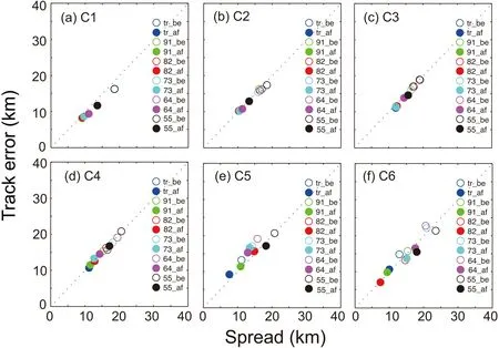
Fig.1.Scatterplots of Maria in 6-h cycles (from 0700 to 1200 UTC 8 July 2018).The X-axis represents the ensemble spread (units:km) and the Y-axis represents the track errors (units:km).“be”and“af”represent before and after sample optimization.“82_be”means before sample optimization in the“82”scheme.“64_af”means after sample optimization in the“64”scheme.

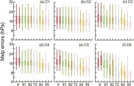
Fig.2.Boxplots of Haima in 6-h cycles (from 1900 UTC 18 October to 0000 UTC 19 October 2016).The X-axis represents the six schemes,the Y-axis represents the absolute errors in MSLP (units:hPa).The front and the following boxes with the same color represent before and after sample optimization,respectively.

Figure 3 shows the maximum wind speed (MWS)errors of TC Hato (201713) over 6-h cycles.The maximum values were reduced from C1 to C6.The range of“73”was reduced most in C4 and C5.However,the range of“82”showed the most reduction in C6.The 60 members had the most concentrated distribution in the“82”scheme.Overall,the absolute errors and ranges decreased from C1 to C6 in all schemes,but the different optimal proportions of intensity and track did not bring stability to the change of MWS.

Figure 4 shows the absolute errors of MWS for TC Merbok (201702) in 6-h cycles.The maximum MWS dropped noticeably in C1,in all schemes.The ranges were reduced in C3,except for the“55”scheme.The reduction of the range was largest in the“tr”experiment.The minimum MWS was reduced substantially in“64”and“55”in C5 and C6.Overall,the dispersion reduced from C1 to C6 in all schemes,except“55”.The MWS by“tr”was the most concentrated in the last cycle,moreover,the“tr”scheme had the smallest median.

In general,sample optimization had some effect on adjusting the MWS indirectly,and reduced the range and spread of MWS.However,there was no obvious pattern for the changes in MWS distribution among the different optimal schemes.

3.2.Structural Adjustment

The structure of TCs should be analyzed to better understand how to combine the two criteria (the observed track and intensity) to achieve better simulations.Considering the length limit of the article,Ewiniar (201804) is deemed to be a representative TC and its structural changes will be shown.The vertical structures of Ewiniar (201804) are displayed in Figs.5 and 6.The starting point (0) of the x-axis represents the calculated typhoon center.The value of each altitude layer was taken as the average radius.The simulation results were compared with the ECMWF analysis field.Although the ECMWF analysis field may not perfectly reproduce the inner core structure of TCs because the number of assimilated observations was limited,there was no better available data than the ECMWF analysis field close to the observation.

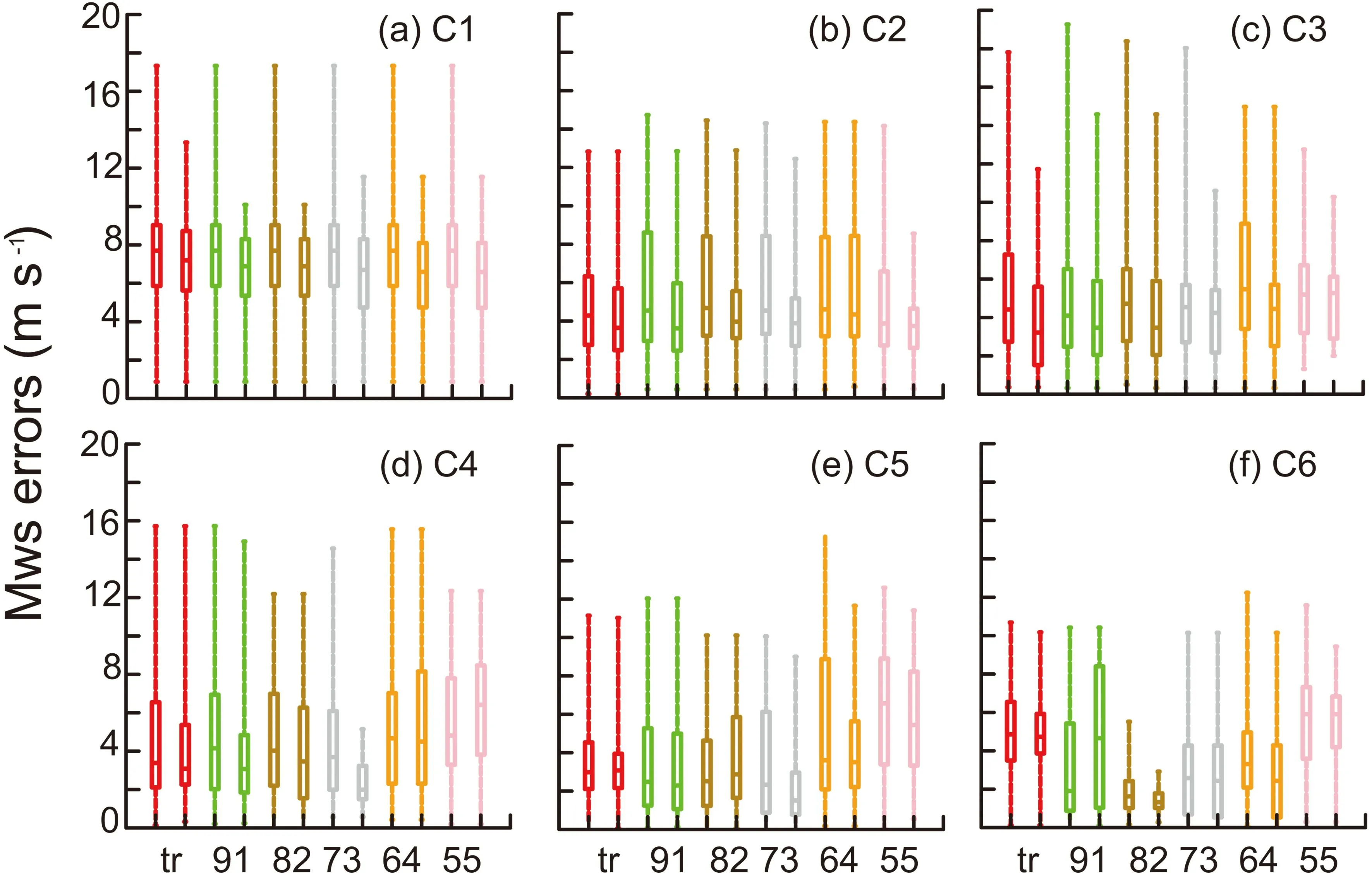
Fig.3.Boxplots of Hato (from 1000 to 1500 UTC 21 August 2017).The X-axis represents the six schemes,the Yaxis represents the absolute errors of the MWS (units:m s-1).The front and the following boxes with the same color represent before and after sample optimization,respectively.

Fig.4.Boxplots of Merbok (from 1900 UTC of 10 June to 0000 UTC of 11 June 2017).The X-axis represents six schemes and the Y-axis represents the absolute errors of the MWS (units:m s−1).The front and the following boxes with the same color represent before and after sample optimization,respectively.

The changes in the thermal and dynamic fields of Ewiniar (201804) were analyzed in Fig.5.The temperature anomaly at each vertical layer is the difference between the temperature at that point and the mean temperature at the same layer.From Fig.5,the potential vorticity of Ewiniar(201804) in the analysis field was significantly weaker than that in SOno near 800 hPa.Sample optimization effectively reduced Ewiniar (201804)’s potential vorticity.When the proportion of the observed intensity became larger in the sample optimization schemes,the potential vorticity had been strengthened in the middle or upper layer by“64”and“55”.Considering both intensity and shape distribution of potential vorticity,“91”and the analysis field had the highest similarity.Next,the influence of sample optimization on Ewiniar (201804)’s thermal structure was analyzed.Compared with SOno,sample optimization improved the structure of Ewiniar (201804)’s warm core and effectively reduced its intensity.When the proportion of observed intensity was over 30% in sample optimization (“73”,“64”,and“55”),the warm core in the upper layer was closer to the analysis field.Thus,with the increased proportion of intensity,the influence of TCs on the thermal structure may be more obvious.

Figure 6 shows the changes in the vertical wind field of Ewiniar (201804).There was a clear outflow at a radial distance of 120 km at 600 hPa in the analysis field,while the upper and lower layers were both dominated by inflow.However,the simulation results of SOno were almost opposite,which had an outflow at the lower layer,but an inflow at the upper layer,which supports the premise that the vertical structure had a beneficial adjustment by sample optimization.With the proportion of the observed intensity increased in sample optimization schemes,the outflow became stronger than the analysis field below 600 hPa.It can be seen that the radial wind simulated by“91”was a little better than the other schemes,which may support the improved prediction of the track of Ewiniar (201804) later in its life cycle.Similarly,the tangential winds simulated by sample optimization were still better than SOno,especially,“tr”,“91”,“64”,and“55”,which outperformed the other schemes and had high similarity with the analysis field.However,when the radius was larger than 300 km,the tangential wind simulated by“tr”and“91”were stronger than the analysis field,meanwhile,the tangential wind simulated by“64”and“55”were weaker than the analysis field.

Figure 7 shows the horizontal wind speed of Ewiniar(201804).The wind speed distribution of Ewiniar (201804)in the analysis field was asymmetric.The wind speed in the southeast quadrant of Ewiniar (201804) was stronger than that in the northwest (Fig.7a).The intensity of Ewiniar(201804) simulated by SOno was notably stronger (over 3–4 m s) than the analysis field,and the typhoon eye had a large position deviation.However,the position and intensity of simulated Ewiniar (201804) were not noticeably improved by“tr”.Fortunately,when intensity was taken into account as selection criteria,the simulated intensity of Ewiniar (201804) was evidently weakened by sample optimization.When the proportion of the observed intensity increased,the intensity of Ewiniar (201804) went through the process of rising and falling.When the proportion of the observed intensity was over 40% in sample optimization(“64 ”and“55 ”),the intensity of simulated Ewiniar(201804) was weaker than the analysis field.On the whole,“91”and“82”outperformed the other schemes in adjusting the horizontal wind field of Ewiniar (201804).

Fig.5..The temperature anomaly (black contoured) (units:°C) and potential vorticity (shaded) (PVU) of Ewiniar with height (units:hPa) and radius (units:km) at 1200 UTC 4 June 2018,(a) analysis,(b) SOno,(c) tr,(d) 91,(e) 82,(f) 73,(g) 64,(h) 55.

Figure 8 shows the sea level pressure,500 hPa geopotential height,and Ewiniar (201804)’s location at different times.The positions at the 0-h forecast by“tr”and "91"were similar.The simulations of Ewiniar (201804) by SOno and“tr”were stronger than the analysis field.When the optimization standard considered the intensity,Ewiniar (201804)’s simulated intensity decreased profoundly by“91”.It can be seen from the analysis field that as Ewiniar (201804)stretched upward,it tilted westward,which was best described by“91”.Furthermore,the track prediction by“91”was better than“tr”.This indicates that the improvement of initial intensity and structures may also have a positive effect on track prediction,which was well confirmed in Ewiniar (201804)’s track error comparison.

4.Analysis of Experimental Results

4.1.Track Prediction

The error,spread,and structural changes in 6-h cycles by the seven schemes were compared,and then the simulation results were analyzed.

Fig.6.The radial (shaded) and tangential (black contoured) wind (units:m s−1) of Ewiniar with height (units:hPa)and radius (units:km) at 1200 UTC 4 June 2018,(a) analysis,(b) SOno,(c) tr,(d) 91,(e) 82,(f) 73,(g) 64,(h) 55.

Figure 9 shows that the simulated TC tracks by each of the seven sample optimization schemes were similar to that of the observed track.Figure 10 displays the quantitative analysis of the experimental results.Among the seven schemes,“tr”had the lowest mean track errors in 6 h and 48 h (in Fig.10a and Fig.10d),“55”had the lowest mean track error in 12 h (Fig.10b),and“91”had the lowest mean track error in 24 h (Fig.10c).The mean track errors simulated by“tr”were smaller compared to“SOno”in 6,12,24,and 48 h,which outperformed the other schemes.The mean track errors simulated by“55”and“91”were three times smaller than those of“SOno”and had good performances.It is worth mentioning that the mean track errors simulated by all schemes were smaller than“SOno”in 48 h.Finally,the higher the proportion of the observed track in the criterion of sample optimization,the better the performance in the track simulation.

4.2.Intensity Prediction

The results of intensity prediction were validated.First,we note that“tr”had the worst simulated MSLP among the seven schemes in 6 h and 12 h (Fig.11).Most schemes outperformed SOno except“tr”.The best performance was from“55”and“64”at 6 h and 12 h,respectively.Then,the simulated results changed.The MSLP errors simulated by all sample optimization schemes were smaller than SOno in 24 h,and the best performance was“55”.However,the situation changed dramatically over 48 h.The“tr”,“91”,“82”,and“64”schemes were better than“SOno”in simulating MSLP.The performance of“91”was particularly notable,but“55”was the worst among all experiments.This suggests that the higher proportion of the observed MSLP in the criterion of sample optimization,the more the MSLP simulation improved in the short term.However,the forecast may degrade with evolution.Overall,“91”was better than SOno in all simulations and with the most stable performance.This may be related to good structural adjustment.

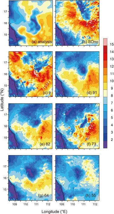
Fig.7.The wind speed (units:m s−1) of Ewiniar at 10 m at 1200 UTC 4 June 2018,(a) analysis,(b) SOno,(c) tr,(d) 91,(e) 82,(f) 73,(g) 64,(h) 55.

Fig.8.The sea level pressure (shaded;units:hPa) and 500 hPa geopotential height (black contour every 10 gpm) at 1200 UTC 4 June 2018,(a) analysis,(b) SOno,(c) tr,(d) 91.Purple and blue filled circles represent the observed and simulated position of Ewiniar for the 0-hour (0 h),12-hours (12 h),24-hours (24 h) forecasts,respectively.

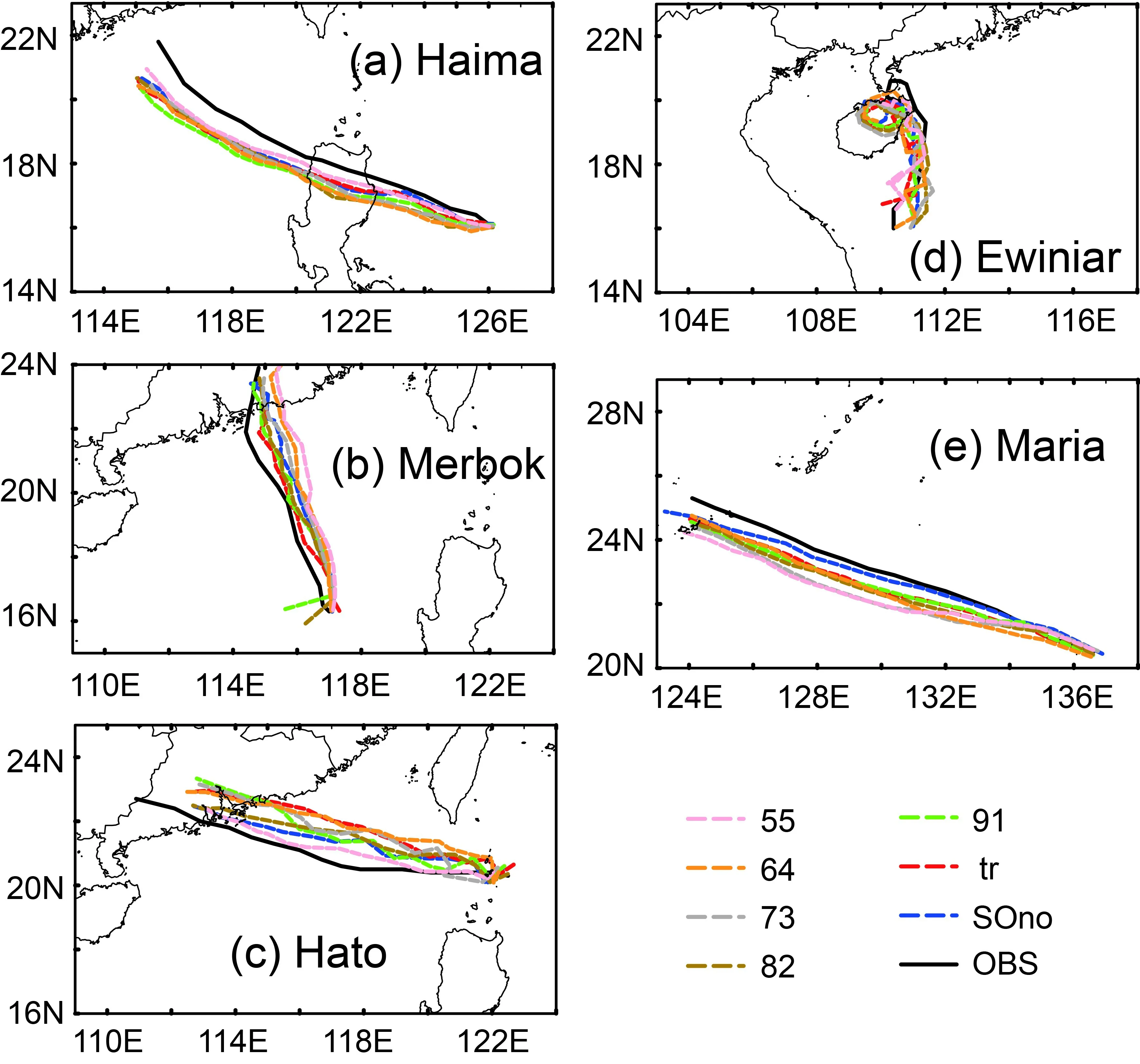
Fig.9.The observed and simulated tracks of five TCs in 48 h.

Fig.10.The track errors of 6-h (a),12-h (b),24-h (c),and 48-h (d),simulations of each TC.

All schemes were worse than SOno when simulating MWS.All schemes were better than SOno in 12 h and the best performance was the“tr”scheme.The MWS simulated by“tr”,“91”,“82”,and“64”were better than“SOno”in 24 h.The performance of“91”was the best,but“73”was the worst among all experiments.Finally,all schemes were better than SOno in 48 h.The“91”scheme had the best performance,and importantly the MWS of“91”was smaller than SOno in all five TC simulations in 48 h.Overall,sample optimization affected the forecast of MWS,but it did not considerably affect the proportion of the observed track and intensity (Fig.12).It is worth noting that“91”was a good performer in terms of MWS prediction.

Fig.11.The absolute errors of MSLP (hPa) of five TCs in 6 (a),12 (b),24 (c),and 48 (d) hours.

Fig.12.The absolute errors in MWS (units:m s−1) of five TCs in 6 (a),12 (b),24 (c),and 48 (d) hours.

5.Summary and Conclusions

According to previous studies,sample optimization of ensemble forecast based only on the observed track had a substantial effect on improving the track prediction of TCs.However,the intensity simulation showed only a slight improvement.Moreover,based only on the observed intensity,the simulation of the intensity was improved by sample optimization to some extent,but the track prediction became worse.To improve the track and intensity prediction of TCs at the same time,the distribution of ensemble members was restricted based on both the observed track and intensity.Then,simulated and observed tracks are compared,and the two indicators are combined to score and rank the sample.When samples with higher scores were obtained,samples with lower scores were eliminated to improve the overall quality of the ensemble forecast.The WRF model was used to simulate five TCs in the northwestern Pacific to test the ability of our scheme to improve the forecast track and intensity of these cyclones.Sample optimization effectively reduced TC track and intensity errors with“55”having better performance on the short-term intensity prediction,and“tr”having better performance on the shortterm track prediction.Considering both track and intensity simulations,“91”was the best and most stable scheme.That is to say,in the actual operational TC forecast,the proportion of A set to 90%,and B set to 10% may yield the best forecast results.

However,it should be noted that the adjustment of TC structures also had an important influence on the simulation of the track and intensity.Although sample optimization(based on both the observed intensity and track) had a positive effect on the improvement of TC structures,there was uncertainty in the adjustment.Moreover,TC tracks are sensitive to internal and external factors.The motion of a TC is driven by the evolution of its intensity,its structure,and its environment.These complex interactions result in a high dependency of TC track predictability on the cyclone features and its environment.From the above analysis,it can be seen that the forecast results of the TCs were closely related to the quality of structural adjustment.Thus,structural similarity should also be taken into account to measure the quality of the sample in future research.Further optimization of the probability distribution of samples may obtain better forecast results.

.The authors would like to thank two anonymous reviewers for their helpful comments,which improved the quality of this paper.This work was supported by the National Key R&D Program of China (Grant No.2018YFC1507602,2017YFC1501603),the National Natural Science Foundation of China (Grant No.41975136),the Guangdong Basic and Applied Basic Research Foundation (Grant No.2019A1515011118),and Scientific research project of Shanghai Science and Technology Commission (19dz1200101).