Probabilistic Load Flow Algorithm with the Power Performance of Double-Fed Induction Generators
2021-09-07CAORuilin曹瑞琳XINGJieHOUMeiqian侯美倩
CAO Ruilin(曹瑞琳) , XING Jie(邢 洁) , 2, HOU Meiqian(侯美倩)
1 College of Information Science and Technology, Donghua University, Shanghai 201620, China
2 Engineering Research Center of Digitized Textile & Apparel Technology, Ministry of Education, Donghua University, Shanghai 201620, China
Abstract: Probabilistic load flow (PLF) algorithm has been regained attention, because the large-scale wind power integration into the grid has increased the uncertainty of the stable and safe operation of the power system. The PLF algorithm is improved with introducing the power performance of double-fed induction generators (DFIGs) for wind turbines (WTs) under the constant power factor control and the constant voltage control in this paper. Firstly, the conventional Jacobian matrix of the alternating current (AC) load flow model is modified, and the probability distributions of the active and reactive powers of the DFIGs are derived by combining the power performance of the DFIGs and the Weibull distribution of wind speed. Then, the cumulants of the state variables in power grid are obtained by improved PLF model and more accurate power probability distributions. In order to generate the probability density function (PDF) of the nodal voltage, Gram-Charlier, Edgeworth and Cornish-Fisher expansions based on the cumulants are applied. Finally, the effectiveness and accuracy of the improved PLF algorithm is demonstrated in the IEEE 14-RTS system with wind power integration, compared with the results of Monte Carlo (MC) simulation using deterministic load flow calculation.
Key words: probabilistic load flow (PLF); cumulant method; double-fed induction generator (DFIG); power performance; series expansion
Introduction
Promoting the vigorous development of renewable energy power generation is a major strategic measure which is taken by most countries in the world to deal with global fossil energy depletion and environmental pollution. Among them, centralized wind power integrated into the grid is one of the main forms of wind energy development and utilization. However, due to the weak controllability and strong randomness of wind power, large-scale wind power integration has brought new challenges to the safe and stable operation of the power grid[1-2].
In order to ensure the safe and stable operation of the system, it is necessary to establish a power grid analysis and calculation method which is suitable for large-scale wind power integration. Probabilistic load flow (PLF) is used to analyze various random factors in the operation of the power system, such as load fluctuations and energy output fluctuations. Statistics theory is used to establish a mathematical model describing the uncertainty and the load flow model of the power system is combined with statistics theory to obtain the steady-state operation of the system[3]. Therefore, a comprehensive PLF algorithm provides more valuable information for reliable and stable operation analysis of power systems. In this paper, the PLF algorithm is improved with introducing the power performance of double-fed induction generators (DFIGs) for wind turbines (WTs).
The cumulant-based expansion is commonly used in PLF algorithm, which mainly includes Gram-Charlier, Edgeworth and Cornish-Fisher expansions. The three kinds of series expansions in operations are all with simplicity and quickness. Gram-Charlier expansion was used in Refs. [4-6] , whose calculation accuracy was almost the same as that of Edgeworth expansion[7], and it is concluded that Gram-Charlier expansion and Edgeworth expansion were identical but each had its own meaning[8]. However, PLF algorithm using Gram-Charlier expansion generates the probability density function (PDF) of the system state variable and the PDF may appear negative values in the tail area. In order to solve the above problems, Refs. [9-10] applied Gram-Charlier expansion of type C to PLF algorithm. Compared with the above two expansions, Cornish-Fisher expansion[7, 11-12]has higher accuracy in calculating the PDF of non-normal distribution. Recently, for the fitting of non-normal distribution, the maximum entropy method[13-15]and the Gaussian mixture model[16-17]have been proposed, but not as good as the series expansion in terms of simplicity and quickness.
In this paper, the power performance of DFIGs for WTs is introduced in the PLF algorithm. DFIG is the main unit type which is used in grid-connected wind farms[1, 18]. Generally, DFIGs have two operation control strategies: the constant power factor control and the constant voltage control. The above literatures usually assumed that the WTs’ active power was defined as a linear function of the wind speed. At the same time, the WTs’ reactive and active power were in a proportional relationship with a constant power factor. These simplifications are not accurate enough to reflect the impact of large-scale integration of WTs on the load flow of the power grid. Therefore, the PLF algorithm for power grid with wind farms is improved by putting the power performance of DFIGs into consideration. In this paper, the conventional Jacobian matrix of the alternating current (AC) load flow model is modified. The probability distributions of the DFIGs’ active and reactive powers are derived according to the power performance of DFIGs under different control strategies.
The paper is organized as follows. In section 1, according to the power performance of DFIGs for WTs under the different control strategies, an AC load flow model including wind farms is built, and the probability distribution of WTs’ output is derived. Section 2 introduces the theoretical background of PLF algorithm by using the cumulant-based expansion. In section 3, based on the IEEE 14-RTS system with wind power integration, the influence of the order of the three cumulant-based expansions on the fitting accuracy of the PDF is compared and analyzed. Additionally, under the different control strategies, the influence of the integration of the DFIGs for WTs on the grid voltage profile is further analyzed. Finally, the conclusions are drawn in section 4.
1 Mathematical Model
1.1 AC load flow model including wind farms
The AC load flow model of the power system is solved by Newton-Raphson iteration method. For a power grid containing wind farms, the linearized correction equation is expressed as
(1)
whereΔPiandΔQiare the errors of active and reactive powers at each conventional bus (including PQ model, PV model and slack bus model).ΔViandΔδiare the corrections of voltage magnitude and angle at each conventional bus. The subscript w indicates the bus where the wind farm is located.Jis referred to as the Jacobian matrix.
(2)
(3)
1.2 Probability distribution of WTs’ output
It is generally considered that the output of the thermal power plant satisfies the 0-1 distribution, the load satisfies the normal distribution, but the probability distribution of wind farm output should be obtained by combining the probability distribution of wind speed and the power curve of WTs.
The probability distribution of wind speed is generally described by a Weibull distribution[19]. The cumulative distribution function (CDF) of wind speedvis given as
(4)
where the constantskandcare the scale and shape parameters, respectively. The parameters can be obtained by analyzing historical data.
The active power curvePGw(v) of DFIGs for WTs is generally provided the manufacturer, as shown in Fig. 1. ThePGwis 0 when the wind speed is lower than the cut-in wind speedvcior higher than the cut-out wind speedvco.The curve can be modelled as
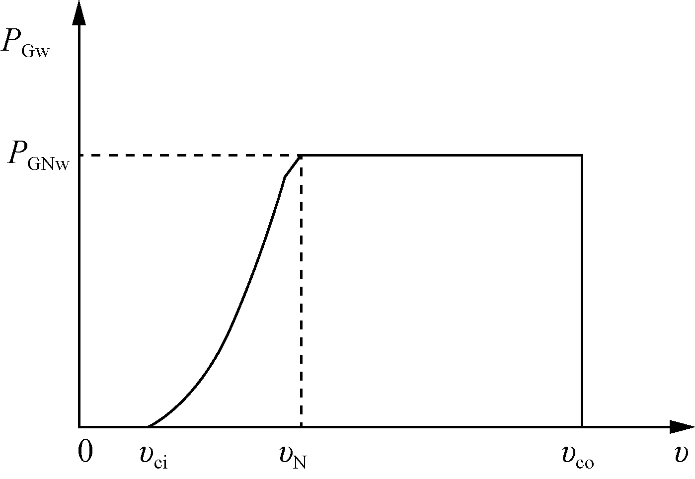
Fig. 1 Active power curve of DFIGs for WTs
(5)
wherevNis the rated wind speed,PGNwis the rated active power, anda0,a1anda2are the coefficients obtained by the least square curve fitting method.
The reactive power curveQGw(Vw,v) of DFIGs for WTs is a function of wind speed and voltage. The DFIGs generate or consume the reactive power. Under the constant power factor control, the flow of reactive power is related to the constant power factor, and under the constant voltage control, it is related to the constant voltage. It can be analyzed that the absolute value ofQGwis the maximum atvNand above, and whenvis lower thanvci, the absolute value ofQGwis the minimum.
The probability distributions of WTs output are expressed as follows.
(1) WhenPGwis 0 or the rated valuePGNw, the probability distribution of the active powerp(PGw) is constant given as
(6)
(2) WhenPGwis between 0 and the rated valuePGNw,p(PGw) is derived from the CDF as

(7)
The probability distribution of the reactive powerp(QGw) is also divided into as follows.
(1)WhenQGwis the minimumQGwminor maximumQGwmax,p(QGw) is constant given as
p(QGw)=
(8)
(2) WhenQGwis betweenQGwminandQGwmax,p(QGw) is derived from the CDF as

(9)
1.3 Power performance of DFIGs for WTs
In this paper, the total power generated by a wind farm is assumed as the sum of power generated by each independent DFIG in the farm, without considering the interaction between WTs. The active powerPGwof a wind farm is a function of wind speed obtained by Eq. (5). The reactive powerQGwof a wind farm is related to the control strategy of DFIGs. When DFIGs are under the constant power factor control, the reactive power of the bus where the wind farm is located is a function of voltage. When DFIGs are controlled by a constant voltage andQGwis within the adjustable range, the bus is set as a PV model in the power flow calculation. But if the reactive power exceeds the adjustable range,QGwas a function of voltage is controlled to the maximum.
The reactive power performance of DFIGs for WTs under the different control strategies mentioned in Ref. [18] is analyzed as follows.

QGw≈Q1=P1tanφ,
(10)
where the relationship between the active powerP1and the reactive powerQ1from the stator side is written as
(11)
wherePGwis obtained by Eq. (5),R1andX1are the stator resistance and reactance,R′2is the reduction value of the rotor resistance ,Xmis the excitation reactance, andsis the slip.
The constant voltage control, which is another common control strategy of DFIGs, is rarely analyzed in the PLF. The voltage amplitude value of a bus where the wind farm is located is a controlled constant by adjusting the reactive powerQGwof DFIGs. The relationship betweenP1andQGwis expressed as
(12)
whereI′2is the reduction value of the rotor current.
As seen from Eq. (12) , the reactive powerQGwis limited by the maximum currentI′2mof the WT rotor-side converter, and the following two cases are discussed.
(1) The reactive power is within the adjustable range. In this case,Vwcan be controlled to be a constant, the bus where the wind farm with DFIGs is located serves as a PV model.
(2) The reactive power regulation exceeds the maximum current limit. WhenI′2reaches the maximum limitI′2m, the left part of Eq. (12) is still greater than the right. In this case, the bus cannot be set as a PV model. The function between the reactive powerQGwand the voltageVwis derived from Eqs. (11)-(12), andI′2=I′2m.
2 PLF Algorithm with Improved Cumulants
The process of PLF algorithm using the cumulant-based expansion can be summarized as follows. Firstly, according to the PDF of the injected power with thermal power plants, wind farms and loads, the cumulants of the injected are obtained. Secondly, the AC load flow calculation is run at the expected value of the injected, andJis calculated by Eq. (1). Then, the cumulants of the power grid state variables are solved by the injected cumulants andJ. Finally, the PDF of the state variable is calculated by series expansion based on the state variable cumulants.
The main steps of the PLF algorithm based on improved cumulants with the power performance of DFIGs are shown in Fig. 2.
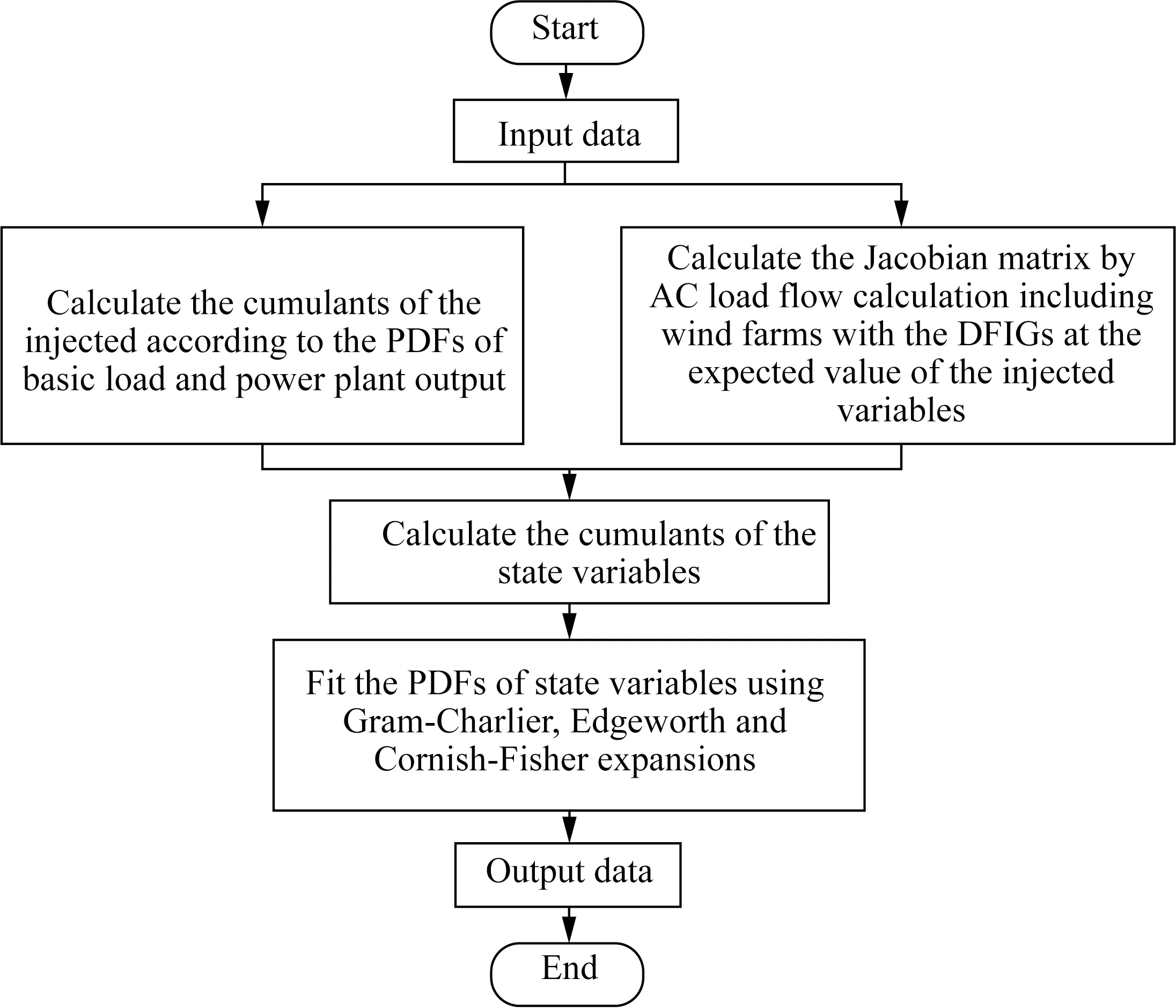
Fig. 2 Flow chart of the proposed PLF algorithm
The theoretical background about cumulant and series expansion introduced below will be applied in this process of PLF algorithm.
2.1 Characteristics of cumulant
The definition of the cumulantkrof each orderris[8]
(13)
where the momentμrof each orderris calculated by the probability distribution of the random variablesx. Ifxis a continuous random variable satisfying the distribution functionF(x), its moment about the mean can be obtained by

(14)
Ifxi(i=1, 2, …,n) is a discrete random variable, and its frequency function isp(xi)(i=1, 2, …,n), its moment is obtained by
(15)
Applying the above theoretical background and Eqs. (6)-(9), the moments of WTs output are obtained by

(16)

(17)
In the PLF algorithm, the cumulant of the injected power is the error of power in AC load flow model and the cumulant of the state variable is the correction. The AC load flow model in PLF algorithm is expressed as
ΔX=J-1ΔW,
(18)
whereΔWis the cumulant of the injected variable,ΔXis the cumulant of the state variable.
The random variables injected into the grid are assumed as independent of each other. According to the properties of the cumulant, the following conclusions can be obtained[20].

(19)
(2) TheΔXrof each orderris obtained by
ΔXr=(J-1)rΔWr.
(20)
2.2 Series expansion
The following three series expansions based on the cumulants are used to obtain the PDF of the state variable in the paper.
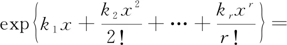
(1) Gram-Charlier expansion[8]is expressed as
(21)
(2) Edgeworth expansion[8]is expressed as
(22)
(3) Cornish-Fisher expansion[10]is expressed as
(23)
In Eqs. (21)-(23),α(x) is the PDF of the standardized normal frequency function,xis a random variable in standard measure.

3 Case Study
The improved PLF algorithm has been implemented in MATLAB and it is tested by using IEEE 14-RTS system. The system diagram is shown in Fig. 3, where the bus1 represents the slack bus, and the generator at the bus2 is set as a wind farm with 20 identical 2 MW DFIGs. The parameters of the DFIG are as follows:R1=0.006 2 Ω,X1=0.002 4 Ω,Xm=4.223 3 Ω,R′2=0.002 4 Ω,X′2=0.069 4 Ω, ands=-0.208.The DFIG’s standard power curve is modelled as Eq. (3), in whichvci=3 m/s,vco=25 m/s,vN=10.8 m/s,PGNw=2 MW,a0=87,a1=-110 anda2=27.

Fig. 3 Diagram of IEEE 14-RTS system
The probability distributions in the test are Weibull distribution of wind speed, 0-1 distribution (2% outage rate) of the thermal power plant output and the normal distribution (the standard deviation is 30% of the expected value) of the load.
In case study, the improved PLF algorithm results are analyzed by comparing with the results from Monte Carlo (MC) simulation. The power values from each distribution are randomly selected in MC simulation, and a total of 20 000 sets of data are selected. Each set of data is substituted into the deterministic AC load flow calculation. Finally, the 20 000 sets of results obtained by multiple iterations are drawn as a reference for the curves of the results from PLF.
In order to compare the accuracy of the results at different series expansions in a clearer way, the average root mean square (ARMS) is introduced as the accuracy reference, obtained by
(24)
whereLiis the value ofith point on the PDF curve calculated by the PLF algorithm,Miis the value ofith point on the PDF curve obtained by the MC simulation, and the number of pointsN=20 000.
3.1 Comparison of the results of different series expansions
When the wind farm in test system adopts the constant power factor control (cosφ=0.98,φ<0) and wind speed satisfies Weibull distribution withk=2.84 andc=7.35, the results obtained by the PLF algorithm with different series expansions of 5-order are compared in Fig. 4. Figures 4 (a) and (b) show the PDFs of bus2 and bus9 voltages, respectively.

Fig. 4 PDFs of the nodal voltage at different series expansions (p.u. means per unit)
The wind farm in test system adopts the constant power factor control (cosφ=0.98,φ<0) and wind speed satisfies Weibull distribution with two cases. One isk=2.84 andc=7.35, and the other isk=1.50 andc=10.70.The results obtained by different series expansions of different orders are compared in Table 1, where ARMS average values of the PDFs of the nodal voltage are shown.
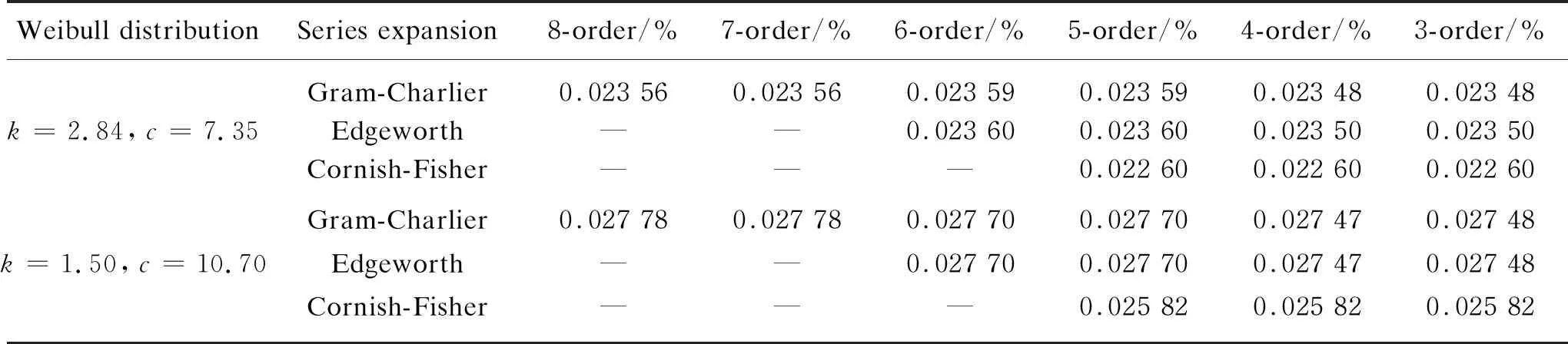
Table 1 ARMS average values of the PDFs of the nodal voltage
From Fig. 4 and Table 1, the PLF algorithm results with the three series expansions are all very close to the results obtained by the MC simulation, so the PLF algorithm using the cumulant-based expansion is accurate enough. In addition, it concludes that the order of the expansion of each level has impact on the obtained PDF. When the expansion order increases, the error tends to increase, as mentioned in Ref. [8] that Edgeworth expansion is usually not higher than 6-order. Overall, the PLF algorithm using the Cornish-Fisher expansion leads to a higher accuracy, and the deviation between its results and the MC simulation results is minimal.
3.2 Impact of wind farms with DFIGs under different control strategies on grid
The impact of integrating wind farms with DFIGs under different control strategies on the grid is analyzed by the improved PLF algorithm using the 5-order of Cornish-Fisher expansion. The PDFs of nodal voltages in the test system are compared in Fig. 5. There are three cases. In case 1, the generator at bus2 is a wind farm with DFIGs under the constant power factor control (cosφ=0.98,φ>0). In case 2, the generator at bus2 is a wind farm with DFIGs under the constant voltage control. The generator at bus2 is a 40 MW thermal power plant in case 3.

Fig. 5 PDFs of the nodal voltage at different cases (p.u. means per unit)
Figures 5 (a) and (b) show the PDFs of bus4 and bus7 voltages, respectively. When the wind farm with 20 identical 2 MW DFIGs replaces a 40 MW thermal power plant, the voltage at each bus in grid moves in a decreasing direction. Additionally, under different control strategies, the voltage variation range of each bus is the same, but the wind farm controlled by the constant voltage has less impact on the grid. When the DFIGs are under the constant voltage control, the part of the nodal voltage PDF curve that rises in the positive direction is very close to the PDF curve in the case of thermal power plant connected. By comparing Figs. 5 (a) and (b), we can see bus4, which is closer to the wind farm connection point, is impacted more in terms of voltage profile.
4 Conclusions
The improved PLF algorithm in this paper uses the cumulant-based expansion with the power performance of DFIGs for WTs. In the proposed algorithm, the power performance of DFIGs is analyzed under the constant power factor control and the constant voltage control. Then, the Jacobian matrix is modified accordingly in the AC load model and the probability distribution of WTs’ output is derived. The improvement makes the results of PLF algorithm more accurate in theory. The effectiveness and accuracy of the improved PLF algorithm using Gram-Charlier, Edgeworth and Cornish-Fisher expansions is demonstrated respectively and compared in the IEEE 14-RTS system. In addition, the impacts on the grid voltage profile of integrating wind farms with DFIGs under the constant power factor control and the constant voltage control are analyzed and compared with integrating the thermal power plant with equal capacity. The conclusions of case studies can be summarized as follows.
(1) The results of the improved PLF algorithm using the cumulant-based expansion are very close to the results obtained by the MC simulation, among them, Cornish-Fisher expansion’s result provides the best accuracy.
(2) The order of series expansion has impact on the fitting result of PDF, so the order should not be too high.
(3) Replacing a thermal power plant with DFIGs in equal capacity makes the voltage magnitude of each bus in the grid decrease, and under the two control strategies the bus voltage variation range is the same.
杂志排行

Journal of Donghua University(English Edition)的其它文章
- Surface Modification of Electrospun Poly(L-lactide)/Poly(ɛ-caprolactone) Fibrous Membranes by Plasma Treatment and Gelatin Immobilization
- Outage Probability Based on Relay Selection Method for Multi-Hop Device-to-Device Communication
- Channel Characteristics Based on Ray Tracing Methods in Indoor Corridor at 300 GHz
- Electromagnetism-Like Mechanism Algorithm with New Charge Formula for Optimization
- Prediction of Online Judge Practice Passing Rate Based on Knowledge Tracing
- Raoultella terrigena RtZG1 Electrical Performance Appraisal and System Optimization