Numerical Modelling for Dynamic Instability Process of Submarine Soft Clay Slopes Under Seismic Loading

MI Yang, WANG Jianhua, *, CHENG Xinglei, and YAN Xiaowei

Numerical Modelling for Dynamic Instability Process of Submarine Soft Clay Slopes Under Seismic Loading

MI Yang1), 2), WANG Jianhua1), 2), *, CHENG Xinglei1), 2), and YAN Xiaowei1), 2)

1),,300072,2),,300072,

Marine geological disasters occurred frequently in the deep-water slope area of the northern South China Sea, especially submarine landslides, which caused serious damage to marine facilities.The cyclic elastoplastic model that can describe the cyclic stress-strain response characteristic for soft clay, is embedded into the coupled Eulerian-Lagrangian (CEL) algorithm of ABAQUS by means of subroutine interface technology. On the basis of CEL technique and undrained cyclic elastoplastic model, a method for analyzing the dynamic instability process of marine slopes under the action of earthquake load is developed. The rationality for cyclic elastoplastic constitutive model is validated by comparing its calculated results with those of von Mises model built in Abaqus. The dynamic instability process of slopes under different conditions are analyzed.The results indicate that the deformation accumulation of soft clay have a significant effect on the dynamic instability process of submarine slopes under earthquake loading. The cumulative deformation is taken into our model and this makes the calculated final deformation of the slope under earthquake load larger than the results of conventional numerical method. When different contact conditions are used for analysis, the smaller the friction coefficient is, the larger the deformation of slopes will be. A numerical analysis method that can both reflect the dynamic properties of soft clay and display the dynamic instability process of submarine landslide is proposed, which could visually predict the topographies of the previous and post failure for submarine slope.

submarine slope; saturated soft clay; coupled Eulerian-Lagrangian; cyclic elastoplastic model; dynamic instability process

1 Introduction

The deep-water slope region in the northern part of the South China Sea is an important region for offshore gas and oil exploration, and it is also a high-risk region for sub- marine landslides (Zheng and Yan, 2012; Li, 2013; Sun and Huang, 2014). Submarine landslides are the major threat to marine structures such as submarine pipelines (Dong, 2017; Guo, 2018; Nian, 2018; Dutta and Hawlader, 2019). The factors triggering submarine landslide include earthquake, decomposition of carbohydrate, liquefaction of sandy soil and weakening of sensitive clay strength. Previous studies have indicated that earthquake load is a significant factor in triggering submarine landslides (Fine., 2005; Masson., 2006). Therefore, the study of the dynamic destabilization process for submarine slopes under the action of seismic loading is essential for the planning and designing of ocean engineering.

In previous studies, many scholars adopted stress-deformation analysis methods to know about the deformation and instability processes of slopes under the action of gravity (Crosta., 2003; Bui., 2008, 2011; An- dersen and Andersen, 2009; Zhang, 2014, 2017, 2018, 2019; Nonoyama, 2015; Sun and Song, 2015; Hu, 2016; Shi, 2018, 2019; Tang, 2018). While, there are few studies about the dynamic instability process for submarine landslide under earthquake loading in previous studies.Jiang. (2018) employed the coupled CFD-DEM method to examine the dynamic instabi- lity process triggered by earthquake load for the methane- rich marine slope, but did not take into account the dynamic properties of submarine landslide materials.Xu(2013) used the display algorithm of Abaqus to analyze the destabilization process of Tangjiashan landslide under seismic loading, predicted the topography and sliding dis- placement of landslide before and after the earthquake.However, the dynamic characteristics of landslide materials are not considered. Biscontin(2004) employed the finite element method to examine the seismic response of a one-dimensional infinite gentle slope. The constitutive model used by Biscontin. (2004) can only predict the deformation of slope under one-dimensional cyclic shear loading, but the deformation under the general stress state was not analyzed and the dynamic instability process of submarine slope could not be described. Zhou(2017) analyzed a sensitive clay marine slope with strain softening characteristics under seismic load. It was concluded that the change of soil properties after disturbance of sensitive clay has an important effect on the dynamic response for marine clay slope. The cumulative deformation is also predicted, but the dynamic properties of the slope soil mass are not considered. Azizian and Popescu (2005) analyzed retrogressive failures for sandy marine slopes under earth- quake load by using an element removal method. The failuresoil mass was completely removed by the element removal method, which was different from the actual slope sliding. Bhandari(2016) adopted the material point method (MPM) to investigate the seismic failure process on slopes.The material point method overcomes the problems of nonconvergence and numerical instability encountered in the traditional numerical analysis methods when dealing with large deformation problems. However, the Mohr- Coulomb model could not describe the cyclic hysteretic characteristic and deformation accumulation characteristic of slope soil mass under earthquake loading, so the numerical calculation results are still uncertain.Taiebat(2011) examined the seismic response of the clay slopes by adopting FLAC3D. The shear strain and deformation of clay slopes under the action of seismic load were predicted. However, the analysis method could not reflect the dynamic properties of slope soil mass and the destabilization process of the slope. Hung. (2018) adopted the Mohr-Coulomb model and display the algorithm of Abaqus to investigate the failure process of slope under the action of earthquake loading, but the dynamic properties of slope material are not considered.

In summary, there has been little previous analysis for the dynamic instability process of slopes under earthquake loading. And the few researches are limited to adopt static constitutive models.The difficulty lies in the fact that the existing numerical analysis methods cannot simultaneous- ly reflect the dynamic properties of the slope soil mass and dynamic instability process of slopes under the action of seismic loading. Therefore, it is essential to investigate such numerical analysis methods.

The cyclic elastoplastic model is embedded into the CEL algorithm of the Abaqus platform. On basis of the CEL method and the cyclic elastic-plastic constitutive mo- del, a numerical analysis method for describing the dynamic instability process of slopes is established. Compared with the results of von Mises model embedded in Abaqus, the applicability of cyclic elastoplastic finite element method is verified. And the dynamic instability pro- cess of marine soft clay slopes under different conditions are investigated, and the final sliding distance of the slope is quantitatively predicted, which provides the basis for the planning and designing of ocean engineering.

2 Analysis Technique

The dynamic instability process of slope involves large deformation of landslide materials. However, most of the existing numerical analysis methods are on basis of the traditional Lagrangian framework, and the mesh element is always bound to the material. The mesh deforms with the deformation of the material. Therefore, the numerical calculation will not converge due to the serious distortion of the meshes when dealing with large deformation pro- blems (Griffiths and Lane, 1999). The dynamic instability process of submarine slopes under seismic load was analy- zed by using the CEL method. Eulerian material is adopted to simulate the soil mass of submarine slope, and the dynamic instability process of slope could be investigated. The CEL method is different from the computational fluid dynamics (CFD) method when dealing with Eulerian ana- lysis. The Eulerian time integration in Abaqus finite element program is on basis of the operator splitting algorithmfor the governing equations in computational solid mechanics framework. Each time increment step is decomposed into two calculation stages: Lagrangian analysis stage and Eulerian analysis stage. The governing equations of the coupled Eulerian Lagrangian method are briefly in- troduced (Benson, 1992, 1995; Benson and Okazawa, 2004).

2.1 Governing Equations in Eulerian Lagrangian Formulations

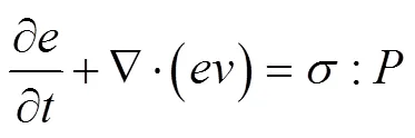
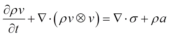
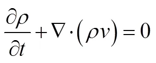
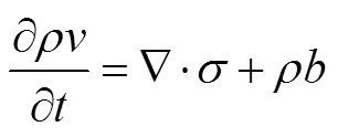
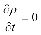
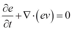
The conservation equations of energy, momentum and mass are generally based on Lagrangian form in the framework of solid mechanics, as shown in Eqs. (1)–(3):

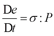
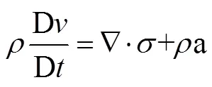
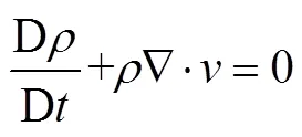
The material time derivative D/Dis described by Lagrangian description, while the spatial time derivative ∂/ ∂is described by Eulerian description.is Cauchy stress tensor,is internal energy,is material density,is phy- sical force,is strain rate,Ñis gradient operator,is the time andis velocity of material.

For an arbitrary variable, the relationship between ma- terial time derivative and spatial time derivative is ex- pressed by Eq. (4).

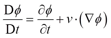
whereÑis the gradient operatorandis the velocity of the material.

Substituting Eq. (4) into Eqs. (1)–(3). The governing equations based on Lagrange framework can be converted to the governing equations described by Eulerian description. And the conservation equations of energy, momentum and mass in space coordinate system are expressed as Eqs. (5)–(7).

The Eqs. (5)–(7) is decomposed into two stages by operator splitting algorithm and the solution procedure for CEL method is shown in Fig.1.

In the Lagrange analysis stage,

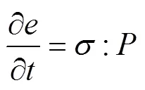
In the Eulerian analysis stage,

, (12)

In the Lagrangian analysis stage, the nodes of the element are temporarily bound to the material, and the mesh deforms with the deformation of the material. The integral solution of Eqs. (14)–(15) is performed in the time increment step by using the display center difference sche- me.

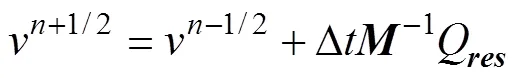
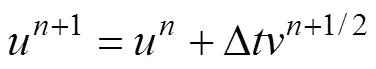
whereandare the velocity and displacement respectively, ∆is a time increment,resis the resultant force vector,is the diagonal concentrated mass matrix and the value of±1/2 is the midpoint of the time increment step.

In the Eulerian analysis stage, the material deformation stops temporarily and the deformed mesh is reshaped to the initial fixed position in Lagrangian analysis stage. The element variables are remapped to the Eulerian mesh by the transport algorithm (Benson, 1992, 1995). The volume of fluid (VOF) method (Benson, 1992) is employed to track the boundary of Eulerian material. In each time incre- ment step, the interface between materials is determined on the basis of the volume fraction of material in the current element and adjacent elements.

2.2 Eulerian Lagrangian Contact

The Eulerian Lagrangian general contact is established by using the penalty function method in the Abaqus CEL finite element method. By introducing the additional stiffness between the surface of Eulerian material and Lagrangian material, the method allows the Lagrangian material to penetrate the Eulerian material. The intrusionis positive, when the Lagrangian material is located inside the Eulerian material. The contact condition must be renewed at each time increment step, which is used to obtain the interaction characteristics between Eulerian material and Lagrangian material. The contact forceFis ex- pressed as Eq. (16):

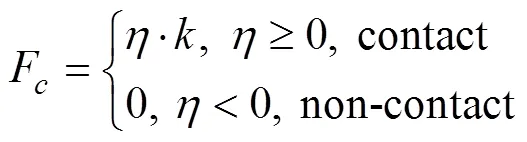
wheredenotes the intrusion distance,denotes the pe- nalty stiffness.

3 Cyclic Elastic-Plastic Constitutive Model

The total volume strain is zero, and the yield and failure of saturated soft clay are independent of volume stress under undrained condition. The evolution of hardening modulus field can be described in deviator stress space, and the cyclic elastic-plastic stress-strain relationship is ex- pressed by total stress. The Mises yield function is used to establish the bounding surface equation (Cheng and Wang, 2016).

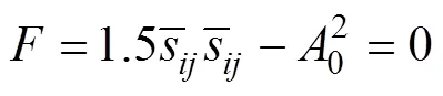
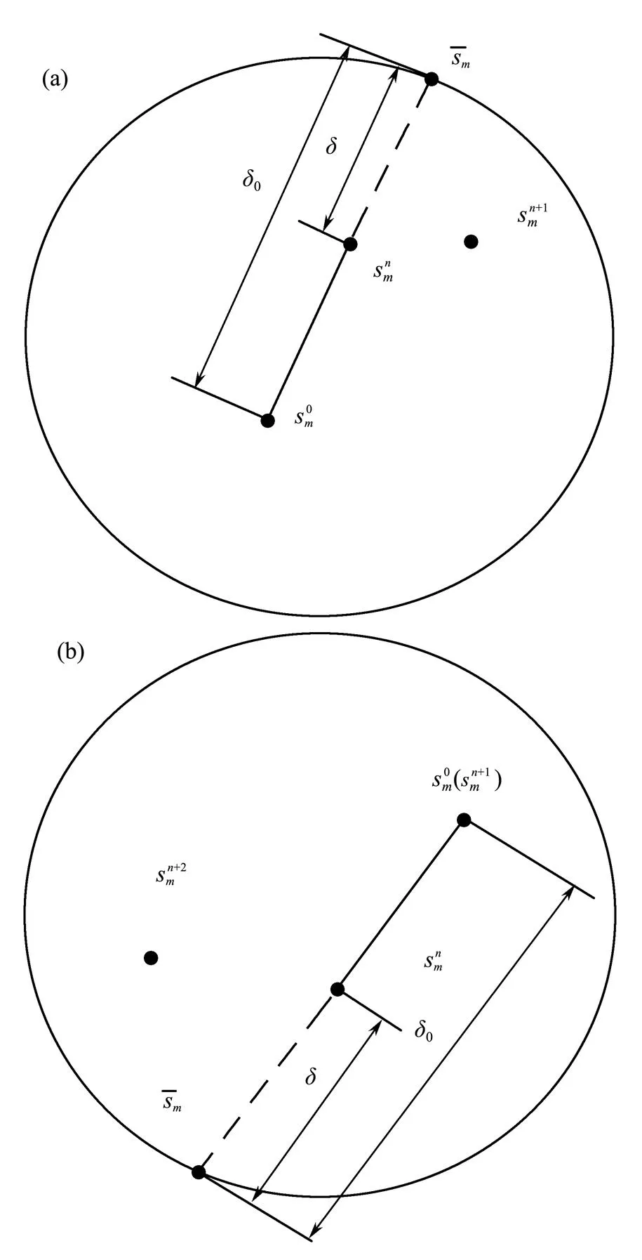
Fig.2 Radial mapping rule. (a), loading; (b), unloading.

The interpolation function of elastic-plastic modulus is described by Eq. (18):

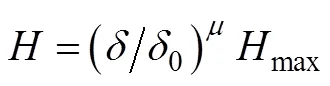
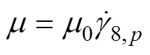
wheredenotes the model parameter that reflects the rate and the magnitude of shear strain accumulation, which can be described as Eq. (19).maxis the maximum value of elastic-plastic modulus.and0are the distances from current stress point and mapping center to the image stress point.

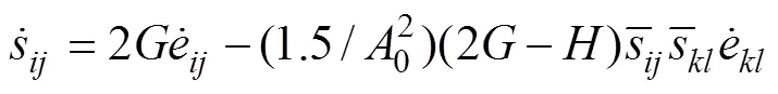
The cyclic elastic-plastic deviatoric stress-strain relationship is described by Eq. (20):

On the basis of elastoplastic theory, the stress increment could be described as Eq. (21):

When considering large deformation problems, the stress- es used in the constitutive relation must be independent of the rotation of rigid body. The differential strain rate of the material needs to be calculated. Jaumann stress rate is described in the form of Eq. (22):

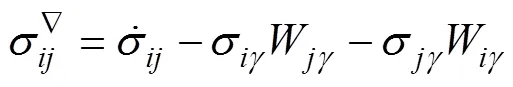
The rotation rate tensor is described in the form of Eq. (23):

The final stress-strain relationship is described as Eq. (24):

According to the radial mapping rule, the elastoplastic modulus interpolation function is established and it is con- sidered that the mapping center moves with the change of loading and unloading paths. Through the interpolation of elastic-plastic modulus and the shift of mapping centers, the evolution law of hardening modulus field is simple, and the parameters used to track the cyclic stress path are less. By introducing parameters that reflect the cumulative mag- nitude and rate of shear strain into the interpolation function of elastic-plastic modulus, the dynamic characteristics of saturated soft clay under the action of seismic load can be described, including the hysteretic, nonlinear and strain accumulation.

where

8, cydenotes the octahedral cyclic shear stress,8, ais the octahedral average shear stress and8fdemotes the octahedral peak shear stress.

4 Numerical Simulation for Submarine Landslide

The undrained cyclic elastoplastic model is embedded in the CEL algorithm of the Abaqus platform. On the basis of CEL method provided by Abaqus platform, the dynamic instability process of submarine landslide under the action of seismic loading is analyzed, and the final sliding distance of submarine landslide is predicted.The proposed method can present the dynamic properties of slope soil mass, can also examine the dynamic instability process of submarine landslide.The physical model description, ana- lysis results and discussion are presented in detail in the following sections.

4.1 Physical Model Description

The CEL method was employed to examine dynamic instability process for the submarine slope and predict the sliding distance of the submarine landslide. The Abaqus CEL framework can only perform three-dimensional numerical simulation analysis. To simplify the analysis, the length of the model in the out-of-plane direction is taken as one element length, which reduces the model to a quasi two-dimensional model deformed in (–) plane. The CEL finite element model consists of three parts: a) a 200H:7V submarine slope, b) void, c) seabed. And the dimensions and mesh of the numerical model are shown in Fig.4.

The material is not always bound to the mesh when the Abaqus CEL method is adopted. When the Abaqus platform is used for post-processing, only the displacement and velocity of the spatial position could be extracted, and the displacement and velocity of the slope soil mass cannot be tracked directly. The tracer particle was defined by modifying INP file, which cannot be defined directly in ABAQUS CAE. By binding the tracer particle with the slope soil mass, the tracer particle can track the movement of the slope soil mass without considering the motion of the mesh. The displacement and velocity of landslide soil are reflected by the displacement and velocity of tracer particles. Tracer particle method is used to track the displacement and velocity at different positions of the submarine slope, which can accurately describe the defor- mation and movement of landslide. Considering the model geometry of the submarine slope, four points at different positions of the slope are selected as the characteristic points for analysis. The distribution of the characteristic points is shown in the Fig.4.

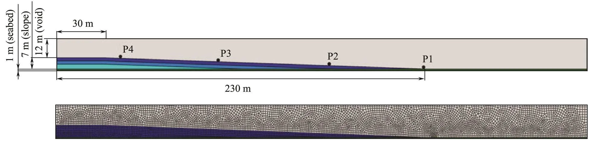
Fig.4 Model geometry and the finite-element mesh.

The submarine slope and void are simulated as Eulerian material and the Eulerian element (EC3D8R) is adopted. In order to simulate the sliding of the submarine slope, the upper and the right part of the slope are set as void space which could accommodate the displaced soil mass. Because the deformation of the seabed is not considered, the three-dimensional eight node solid element (C3D8) is employed to simulate the seabed as a rigid body. A 1m×1m mesh is used for slope and seabed model.The initial conditions of saturated soft clay and void space are set by adopting the Eulerian volume fraction (EVF) tool provided by Abaqus. For the void, EVF=0 and there is no Eulerian material in the Eulerian element. While for saturated soft clay, EVF=1 and Eulerian elements are filled with Eulerian material (saturated soft clay).

Saturated soft clay is assumed to be undrained when the dynamic instability process of submarine landslide is examined, because the permeability coefficient of soft clayis small and the duration for earthquake loading is short.The effects of local drainage and pore water pressure changes on the analysis results were not considered.By assuming undrained condition, the soil-water interaction is somehow considered. And it is a simplified method to consider soil- water interaction. In the finite element simulation, Poisson’s ratio could not be taken as 0.5, so Poisson’s ratio of 0.49 is taken to approximate the undrained condition of saturated clay.The basic physical properties of saturated soft clay on submarine slope are presented in Table 1.

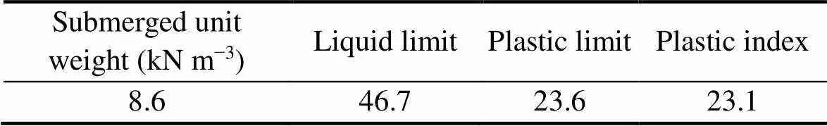
Table1 Basic physical properties of the marine soft clay

In the cyclic elastoplastic constitutive model,0denotes the radius for the boundary surface,is the elastic shear modulus. Here, the values of0andvary almost linearly with the undrained shear strengthS. We assumed that0=2.83S,=29.9S. The relationship of undrained shear strengthSwith depth is described as Eq. (27), whereSincreases almost linearly with depth. The submarine slope model is divided into three layers, each with a thickness of 2m. It is assumed that the strength of each layer is consistent, so the undrained shear strength at the middle position of each layer is taken to be the strength of that clay layer.

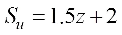
Here,is the depth below the mudline and the un- drained shear strengthSat the mudline is taken as 2kPa.

The general contact condition is used for seabed and slope, and the contact algorithm of penalty function is adopted. The seabed and slope are set as separable contact conditions. The numerical simulation consists of three steps. The first step is the geostatic analysis, which aims to put slope model in the initial stress state. At the end of this step, the slope model is in equilibrium. Then the seismic wave is applied in the form of horizontal acceleration at the bottom of the slope in the second step. The third step is the post-earthquake simulation. The analysis is continued under the earthquake loading until the sliding velo- city of the landslide soil mass is reduced to negligible. There is no velocity boundary condition at the interface between the slope and the void, which allows the displaced soils to move into the void spaces when necessary.The displacement of the seabed is limited and the seabed is not allowed to move during the numerical analysis. The vertical direction of the bottom of the slope, thedirection of the whole model and the external normal direction of all vertical planes are set as zero velocity boundary conditions. To eliminate the reflecting of seismic waves from the truncated boundary, the right side of the slope is set as the nonreflecting boundary. The nonreflecting boun- dary can be directly specified in Abaqus CEL. Thus, the reflection of seismic wave at artificial truncated boundary can be eliminated, and the outgoing wave could be reasonably absorbed.

The 1976 Friuli seismic record is selected as the seismic input, and the revised peak acceleration is 0.35g. The acceleration-time curve is shown in Fig.5.

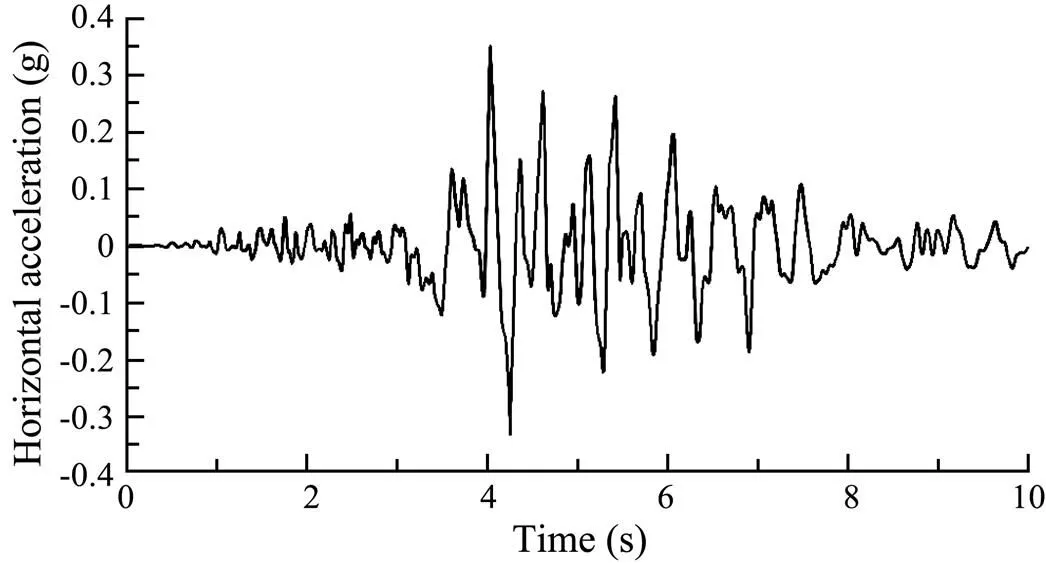
Fig.5 The time curve of horizontal acceleration.

4.2 Analysis Results and Discussion

The dynamic instability process for the slope under the action of the earthquake load is analyzed by CEL method, and the calculation results are compared with those of the von Mises model to verify the applicability of the cyclic elastoplastic constitutive model. Then, the dynamic instability process of the slope under different working conditions are investigated by the cyclic elastoplastic finite ele- ment method. The detailed analysis results and discussion are described below.

4.2.1 Validation of cyclic elastoplastic model applicability

The undrained cyclic elastoplastic model (simulation I) and von Mises model (simulation II) are used to examine the dynamic instability process for submarine landslide under the action of earthquake load.The friction coefficient between submarine slope and seabed is set as 0.5. The relationship between undrained shear strengthSand depth is expressed as Eq. (27), and Poisson’s ratio is 0.49.

When the two constitutive models are used for numerical analysis, the displacement-time curves of different characteristic points are shown in Fig.6. And the curves in simulation I and II are similar.However, the displacement for simulation I is larger than that of simulation II at the end of numerical analysis.In simulation I, the maximum displacement of different characteristic points is about 25.2m, while the maximum displacement is about 17m in simulation II. The final deformation and runout distance are shown as Fig.7. The final deformation and runout distance in simulation I are larger than that of simulation II. The runout distance of the landslide front edge is about 20m in simulation I, while that in simulation II is about 10m.

Therefore, there are differences between the results of simulation I and simulation II.The reason is that when the cyclic elastoplastic model is used to examine the dynamic instability process of slopes, it can describe the cumulative deformation property of slope soil mass under the action of seismic loading. The cumulative deformation characteristic is crucial to the analysis because it may eventually lead to the large deformation in simulation I.The accuracy of von Mises model in Abaqus has been ve- rified in numerical implementation. By comparing the calculation results with the von Mises model, the applicabi- lity of the cyclic elastic plastic model in analyzing the dynamic instability process of submarine slopes is verified.

4.2.2 Cyclic elastoplastic model to simulate the landslide failure

The dynamic instability process of submarine slopes includes downward sliding of clay blocks separated from the slope, and the subsequent sliding of the whole slope along the downslope direction.The separated clay blocks and the soil mass slide forward for a distance along the seabed when the submarine slope is unstable.Therefore, when the roughness of seabed surface is different, the sliding distance will be different.The dynamic instability pro- cess and final sliding distance of submarine slopes are examined by cyclic elastoplastic constitutive model according to different friction coefficients.Li(2011) used the DEM method to examine the instability process for Donghekou landslide, in which the friction coefficient was 0.1–0.5. Shi. (2019) adopted the MPM method to examine the sliding process of 2015 Shenzhen landslide, with friction coefficient of 0.1–0.2.Here, the friction co- efficientsof 0.1, 0.2 and 0.3 are taken for the numerical analysis.

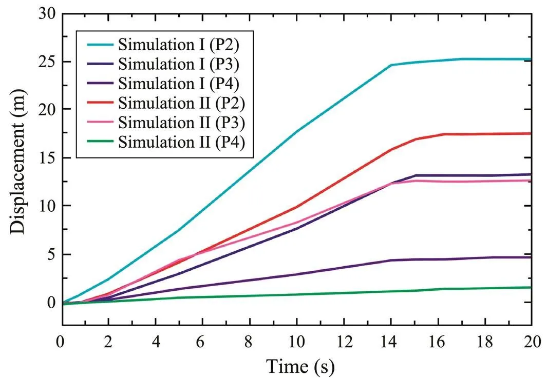
Fig.6 Displacement-time curves of different characteristic points in simulation I and simulation II.

Fig.7 Comparison of submarine landslide topography and runout distance. (a), simulation I; (b), simulation II.

When the friction coefficient is different, the sliding dis- placement and sliding velocity of different characteristic points are different. In Figs.8 and 9, the time curves of sliding displacement and sliding velocity for different cha-racteristic points in the entire sliding process of submarine landslide under different friction coefficients are shown.

As shown in Fig.8, three characteristic points are selected to analyze the sliding displacement under different friction coefficients. The variation trend of sliding displace- ment of characteristic points in the entire sliding process of submarine landslide could be approximately divided into two stages. In the first stage, the slope gradually slides from the initial stable state under seismic loading, and the sliding displacement of the characteristic points increases with the increase of seismic load intensity gra- dually.In the second stage, when the sliding displacement of the characteristic points increases to a certain extent, it gradually tends to be stable. And then, the submarine slope gradually tends to be stable, and finally reaches a new equilibrium state. When the friction coefficients are taken as 0.1, 0.2 and 0.3, the maximum sliding displacement of characteristic point P2 is about 50.3m, 41.5m and 32.5m, respectively.

Fig.9 show that the speed variation trend of feature points could be divided into three stages: at the first stage the speed of different feature points increases gradually; at the second stage the speed approximately tends to be stable; and at the third stage the speed decreases sharply. When the friction coefficient is 0.1, 0.2 and 0.3, the cha- racteristic point P2 reaches the maximum velocity at about=10s, and the maximum velocity is about 3.07ms−1, 2.41ms−1and 2.25ms−1respectively. And then the velocity of the feature points decreases gradually. When the different friction coefficients are selected, the time required for the characteristic points to reach the peak velocity is almost the same. Although the time required for the slope to stabilize is different when different friction coefficients are selected, the velocities of all feature points finally decrease to zero. The submarine slopes gradually tend to be stable and finally reaches a new equilibrium state.

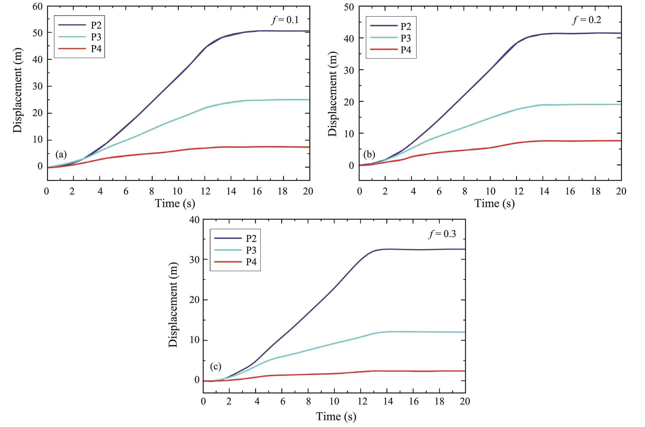
Fig.8 The time curves of sliding displacement for characteristic points P2, P3 and P4 under different friction coefficients.

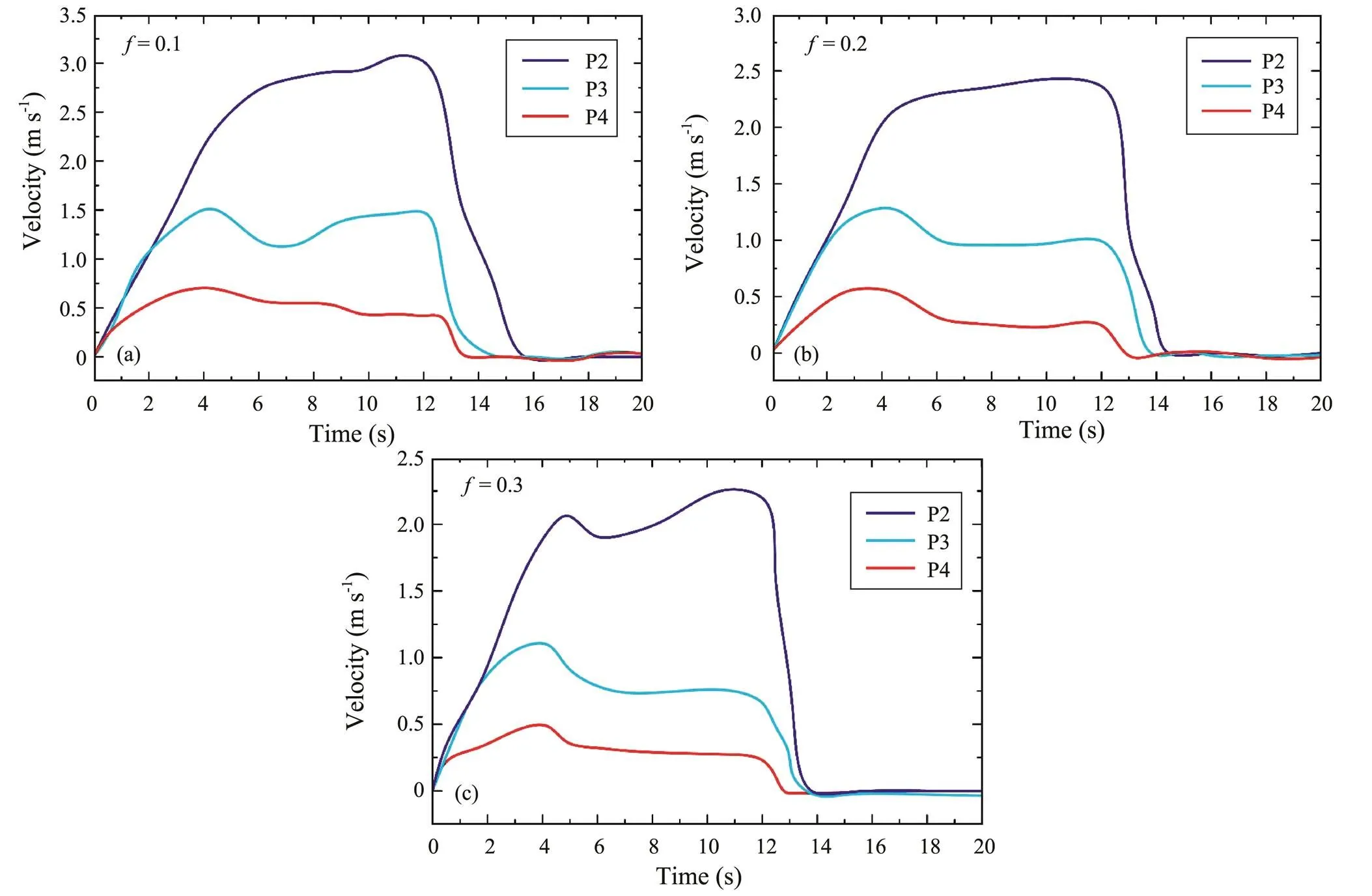
Fig.9 The time curves of sliding velocity for characteristic points P2, P3 and P4 under different friction coefficients.

The final morphology and runout distance of submarine slope after earthquake under different friction coffficients are shown in Fig.10. Figs.7(a) and 10 show that if the friction coffficients are different, the final deformation and runout distance of submarine slope will be different at the end of numerical analysis. Different contact conditions have great influence on the mobility of slope soil mass. When the friction coefficient is taken as 0.5, the final deformation of the submarine slope is relatively small. The runout distance of landslide mass is relatively small, about20m. And the gliding clay block, which is an intact hydroplaning block of cohesive sediment during early stages of landslide, is not completely separated from the landslide mass. Most of the sliding mass is accumulated at the slope toe. While, when the friction coefficient is taken as 0.1, the final deformation of the submarine slope is relatively large. The out-runner clay block is completely separated from the parent submarine landslide mass. The runout distance of the out-runner clay block is about 45m. The final runout distance of landslide mass is about 34m. In other words, the smaller the friction coefficient is, the greater the runout distance and deformation of the landslide will be. Also the glide clay block at the front edge of the landslide will be completely separated from the landslide mass.

The time curves of runout distance for the front edge of landslide (characteristic point P1) obtained by assuming the different friction coefficient is shown in Fig.11. The results show that the smaller the friction coefficient is, the larger the runout distance for leading edge of landslide will be. When the friction coefficient is taken as 0.1, the run- out distance of the front edge of the landslide is the largest, about 45m. And the toe of the submarine slope experienced a significant large deformation during the entire process in the numerical analysis, as shown in Fig.10.

According to the above analysis, the final deformation of submarine slope increases with the decrease of friction coefficient. And the dynamic instability process of submarine slopes is investigated in detail under the friction coefficient of 0.1. In Fig.12 the submarine landslide topography and runout distance at four different moment in the analysis are shown. As shown in the Fig.12(a), the submarine slope is stable at the initial stage, and the slope is not deformed. When=0s, the displacement and velocity of the characteristic points are zero as shown in Figs.8(a) and 9(a). When the earthquake load was put, the displacement and velocity of characteristic points increase gradually with the increase of earthquake load intensity, thus the deformation for sub- marine slope gradually increases. When=5s, the middle part of the slope tends to slide downward, and the clay blocks at the toe of the slope tend to slide away from the submarine slope. After that, the seismic load intensity gradually weakened, but the deformation of the slope con- tinued to increase, and the middle part of the submarine slope keep on sliding downward. When=10s, some glide clay blocks at the toe of the slope slide away from the submarine slope and the deformation of the slope continues to increase. The submarine slope still slides for a certain distance due to the inertia after the end of earthquake. After 10s, the velocity of the landslide mass gradually de- creases to zero, and the sliding displacement finally tends to be stable. Finally, the slope reaches a new equilibrium state and the final stable slope angle is smaller than the initial slope angle.

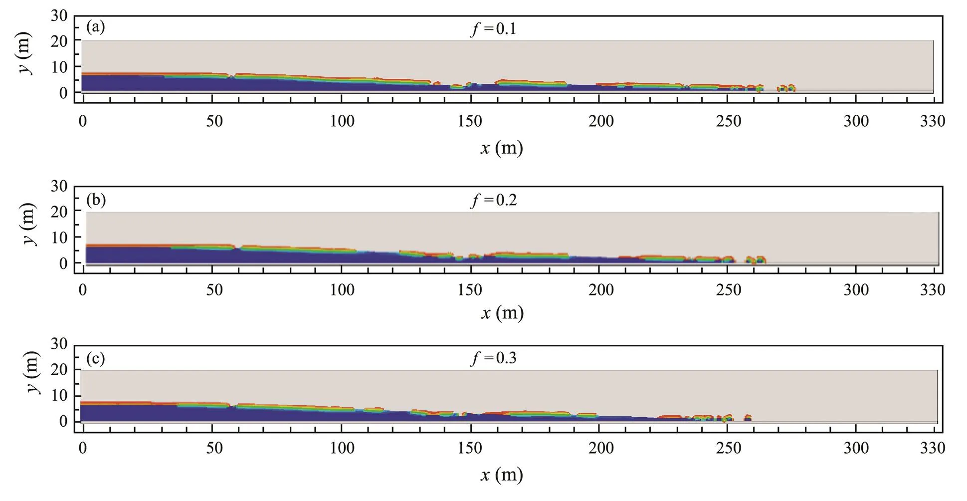
Fig.10 Landslide topography and runout distances simulated by using different friction coefficients.

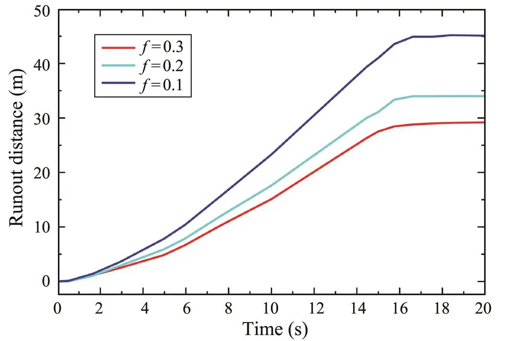
Fig.11 The time curves of runout distance for characteristic point P1 obtained under different friction coefficient.

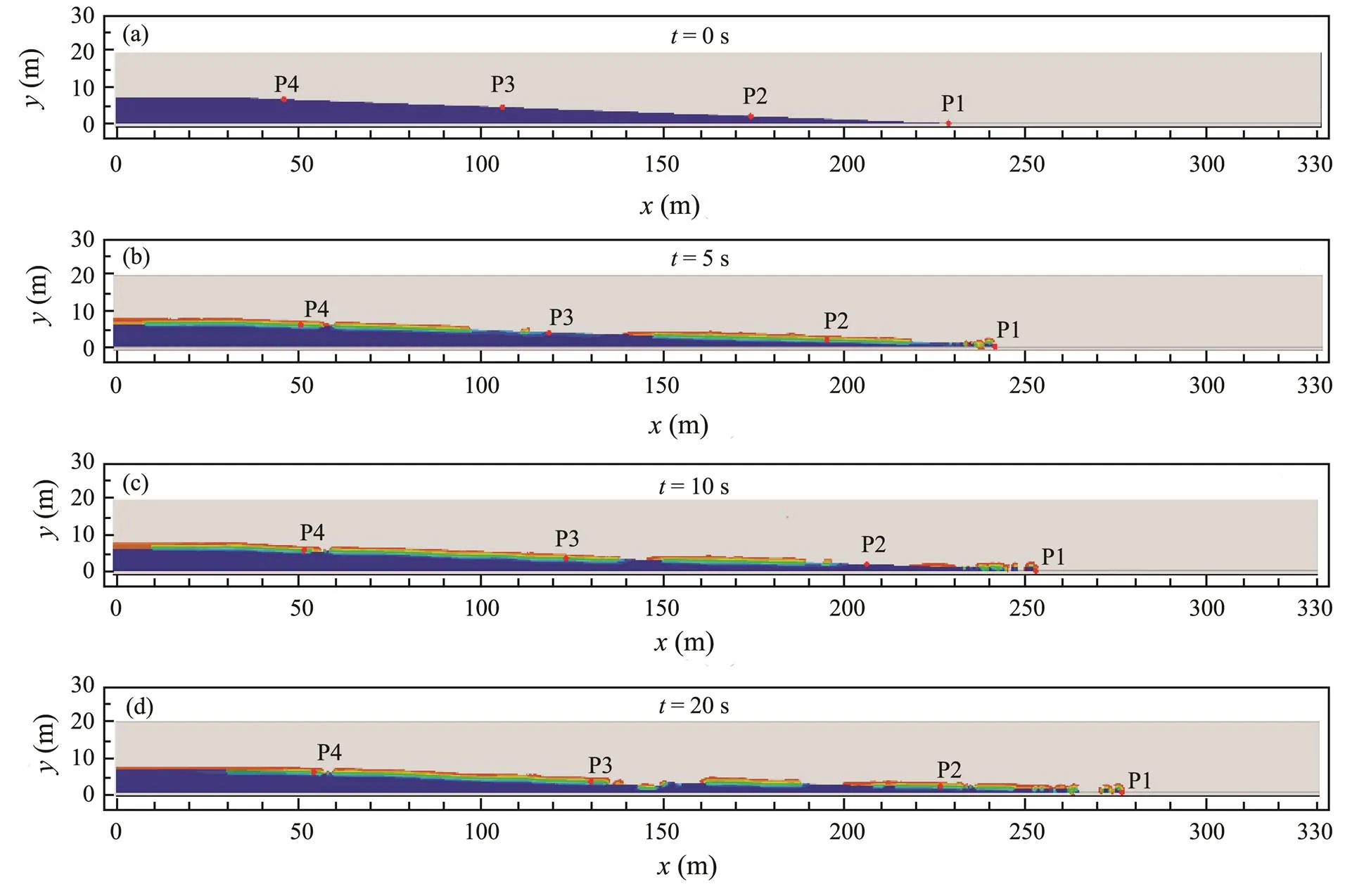
Fig.12 Landslide topography and runout distance at four different time when f=0.1.

4.2.3 Discussion

The above analysis results show that the dynamic instability process of submarine soft clay slopes includes three stages: initial failure stage, deformation and sliding stage and post-failure stage. In the initial failure stage, the sliding of submarine slope is triggered by the seismic load- ing. With the increase of seismic load intensity, the sub- marine landslide gradually enters the stage of deformation and sliding, and the sliding velocity and displacement in- crease gradually. With the gradual weakening of seismic load intensity and the end of the earthquake, the landslide gradually enters the final post-failure stage. The sliding speed of the landslide mass gradually decreases to zero, and all kinetic energy gradually transforms into the deformation. The landslide topography before and after the earthquake indicates that if the friction coefficients are the same, the deformation results calculated by the cyclic elastoplastic constitutive model are larger than that of von Mises model. When the same constitutive model is employed, the smaller the friction coefficient is, the greater the final deformation of submarine slope is.

The results show that the cyclic elastoplastic finite ele- ment method could reflect the entire dynamic instability process of submarine slopes under the action of earthquake load. Compared with the traditional finite element method, the cyclic elastic-plastic finite element method can reasonably reflect the dynamic properties of the soft clay under the action of earthquake loading, and its numerical analysis results are more rational.Therefore, the calculation results acquired by employing the cyclic elastoplastic model are relatively conservative in practical marine engineering applications.

5 Conclusions

The undrained cyclic elastoplastic model is embedded in the coupled Eulerian-Lagrangian (CEL) algorithm of the Abaqus platform. On the basis of CEL method and the cyclic elastic-plastic constitutive model, a numerical analysis method for describing the dynamic instability process of marine slopes is established. Compared with the results of von Mises model embedded in Abaqus, the applicabi- lity of cyclic elastoplastic model is verified. And the dyna-mic instability process of marine slope under different con- ditions are investigated, and the final sliding distance of the slope is quantitatively predicted.

The main conclusions are as follows: 1) deformation accumulation characteristic of slope soil mass has an important influence on the dynamic instability process and makes the deformation and runout distance of submarine landslide larger than that calculated by the traditional static constitutive model; 2)when the von Mises model is used to investigate dynamic instability process of slopes, the final deformation and runout distance of the submarine landslide are underestimated; 3) When different contact conditions are adopted, the smaller the friction coefficient between slope soil mass and seabed is, the larger the final deformation of slope is; 4) The cyclic elastoplastic finite element method could reflect the deformation accumulation characteristic of soft clay, could also visually descri- be the entire dynamic instability process of slopes and to- pographic changes before and after deformation.

In summary, a numerical analysis method that can reflect the dynamic properties of soft clay and the dynamic instability process for submarine slopes is established. It could predict the change of topography before and after the deformation for submarine slopes more intuitively. In addition, it overcomes the drawbacks of traditional numerical analysis methods. Besides, it could solve practical engineering problems conveniently and provide a basis for the planning and designing of marine engineering structures.

Acknowledgement

This work was supported by the National Natural Science Foundation of China (NSFC) (No. 51179174).

Andersen, S., and Andersen, L., 2009. Modelling of landslides with the material-point method., 14: 137-147, DOI: 10.1007/s10596-009-9137-y.

Azizian, A., and Popescu, R., 2005. Finite element simulation of seismically induced retrogressive failure of submarine slopes., 42: 1532-1547, DOI: 10.1139/ t05-032.

Benson, D. J., 1992. Computational methods in Lagrangian and Eulerian hydrocodes., 99: 235-394, DOI: 10.1016/0045-7825 (92)90042-I.

Benson, D. J., 1995. A multi-material Eulerian formulation for the efficient solution of impact and penetration problems., 15: 558-571.

Benson, D. J., and Okazawa, S., 2004. Contact in a multi-ma- terial Eulerian finite element formulation., 193: 4277-4298, DOI: 10.1016/j.cma.2003.12.061.

Bhandari, T., Hamad, F., Moormann, C., Sharma, K. G., and We- strich, B., 2016. Numerical modelling of seismic slope failure using MPM., 75: 126-134, DOI: 10.1016/j.compgeo.2016.01.017.

Biscontin, G., Pestana, J. M., and Nadim, F., 2004. Seismic trig- gering of submarine slides in soft cohesive soil deposits., 203: 341-354, DOI: 10.1016/s0025-3227(03) 00314-1.

Bui, H. H., Fukagawa, R., Sako, K., and Ohno, S., 2008. Lagran- gian meshfree particles method (SPH) for large deformation and failure flows of geomaterial using elastic-plastic soil con- stitutive model., 32: 1537-1570, DOI: 10.10 02/ nag.688.

Bui, H. H., Fukagawa, R., Sako, K., and Wells, J. C., 2011. Slope stability analysis and discontinuous slope failure simulation by elasto-plastic smoothed particle hydrodynamics (SPH)., 61: 565-574, DOI: 10.1680/geot.9.P.046.

Cheng, X., and Wang, J., 2016. An elastoplastic bounding sur- face model for the cyclic undrained behaviour of saturated soft clays., 11: 325-343, DOI: 10.12989/gae.2016.11.3.325.

Crosta, G. B., Imposimato, S., and Roddeman, D. G., 2003. Nu- merical modelling of large landslides stability and runout., 3: 523-538, DOI: 10. 5194/nhess-3-523-2003.

Dafalias, Y. F., 1981. The concept and application of the bound- ing surface in Plasticity theory. In:. Hult, J., and Lemaitre, J., eds., Springer, Berlin, Heidelberg, 56-63, DOI: 10.1007/978-3-642-81582-9_9.

Dong, Y., Wang, D., and Randolph, M. F., 2017. Investigation of impact forces on pipeline by submarine landslide using ma- terial point method., 146: 21-28, DOI: 10. 1016/j.oceaneng.2017.09.008.

Dutta, S., and Hawlader, B., 2019. Pipeline-soil-water interac- tion modelling for submarine landslide impact on suspended offshore pipelines., 69: 29-41, DOI: 10.1680/ jgeot.17.P.084.

Fine, I. V., Rabinovich, A. B., Bornhold, B. D., Thomson, R. E., and Kulikov, E. A., 2005. The grand banks landslide-gene- rated tsunami of November 18, 1929: Preliminary analysis and numerical modeling., 215: 45-57, DOI: 10. 1016/j.margeo.2004.11.007.

Griffiths, D. V., and Lane, P. A., 1999. Slope stability analysis byfinite elements., 49 (3): 387-403, DOI: 10.1680/ geot.1999.49.3.387.

Guo, X. S., Nian, T. K., Zheng, D. F., and Yin, P., 2018. A me- thodology for designing test models of the impact of submarine debris flows on pipelines based on Reynolds criterion., 166: 226-231, DOI: 10.1016/j.oceaneng.2018.08. 027.

Hu, M., Xie, M. W., and Wang, L. W., 2016. SPH simulations of post-failure flow of landslides using elastic-plastic soil constitutive model., 38 (1): 58-67 (in Chinese with English abstract).

Hung, C., Liu, C. H., Lin, G. W., and Leshchinsky, B., 2018. The Aso-Bridge coseismic landslide: A numerical investigation of failure and runout behavior using finite and discrete element methods., 78: 2459-2472, DOI: 10.1007/s10064-018-1309-3.

Jiang, M., Shen, Z., and Wu, D., 2018. CFD-DEM simulation of submarine landslide triggered by seismic loading in methane hydrate rich zone., 15: 2227-2241, DOI: 10.1007/s 10346-018-1035-8.

Li, L., Lei, X., Zhang, X., and Sha, Z., 2013. Gas hydrate and associated free gas in the Dongsha area of northern South China Sea., 39: 92-101, DOI: 10.1016/j.marpetgeo.2012.09.007.

Li, X., He, S., Luo, Y., and Wu, Y., 2011. Simulation of the sliding process of Donghekou landslide triggered by the Wen- chuan earthquake using a distinct element method., 65: 1049-1054, DOI: 10.1007/s12665- 011-0953-8.

Masson, D. G., Harbitz, C. B., Wynn, R. B., Pedersen, G., and Lovholt, F., 2006. Submarine landslides: Processes, triggers and hazard prediction., 364: 2009-2039, DOI: 10.1098/rsta.2006.1810.

Nian, T. K., Guo, X. S., Fan, N., Jiao, H. B., and Li, D. Y., 2018. Impact forces of submarine landslides on suspended pipelines considering the low-temperature environment., 81: 116-125, DOI: 10.1016/j.apor.2018.09.016.

Nonoyama, H., Moriguchi, S., Sawada, K., and Yashima, A., 2015.Slope stability analysis using smoothed particle hydrodynamics (SPH) method., 55: 458-470, DOI: 10. 1016/j.sandf.2015.02.019.

Shi, B. T., Zhang, Y., and Zhang, W., 2019. Run-out of the 2015 Shenzhen landslide using the material point method with the softening model., 78: 1225-1236, DOI: 10.1007/s10064-017-1167-4.

Shi, B. T., Zhang, Y., and Zhang, W., 2018. Analysis of the entire failure process of the rotational slide using the material point method., 18 (8): 1-13.

Sun, Y. J., and Song, E. X., 2015. Simulation of large-displace- ment landslide by material point method., 37 (7): 1218-1225 (in Chinese with English abstract).

Sun, Y., and Huang, B., 2014. A potential tsunami impact assess- ment of submarine landslide at Baiyun Depression in northern South China Sea., 1 (1): 7, DOI: 10.1186/s40677-014-0007-0.

Taiebat, M., Kaynia, A. M., and Dafalias, Y. F., 2011. Applica- tion of an anisotropic constitutive model for structured clay to seismic slope stability., 137: 492-504, DOI: 10.1061/(asce)gt. 1943-5606.0000458.

Tang, Y. F., Shi, F. Q., Liao, X. Y., and Zhou, S., 2018. Determination on flow rules of large deformation analysis of slope based on SPH method., 39 (4): 2-8, DOI: 10.16285/j.rsm.2016.1148 (in Chinese with English abstract).

Xu, W. J., Xu, Q., and Wang, Y. J., 2013. The mechanism of high- speed motion and damming of the Tangjiashan landslide., 157: 8-20, DOI: 10.1016/j.enggeo.2013. 01.020.

Zhang, X., Krabbenhoft, K., Sheng, D., and Li, W., 2014. Nu- merical simulation of a flow-like landslide using the particle finite element method., 55: 167-177, DOI: 10.1007/s00466-014-1088-z.

Zhang, X., Oñate, E., Torres, S. A. G., Bleyer, J., and Krabben- hoft, K., 2019. A unified Lagrangian formulation for solid and fluid dynamics and its possibility for modelling submarine landslides and their consequences., 343: 314-338, DOI: 10.1016/ j.cma.2018.07.043.

Zhang, X., Sheng, D., Sloan, S. W., and Bleyer, J., 2017. Lagran- gian modelling of large deformation induced by progressive failure of sensitive clays with elastoviscoplasticity., 112: 963-989, DOI: 10.1002/nme.5539.

Zhang, X., Sloan, S. W., and Oñate, E., 2018. Dynamic modelling of retrogressive landslides with emphasis on the role of clay sensitivity., 42: 1806-1822, DOI: 10.10 02/nag.2815.

Zheng, H. B., and Yan, P., 2012. Deep-water bottom current re- search in the northern South China Sea., 30: 122-129, DOI: 10.1080/1064119x.2011. 586015.

Zhou, Y., Chen, J., She, Y., Kaynia, A. M., Huang, B., and Chen, Y. M., 2017. Earthquake response and sliding displacement of submarine sensitive clay slopes., 227: 69- 83, DOI: 10.1016/j.enggeo.2017.05.004.

. E-mail: tdwjh@tju.edu.cn

July 30, 2020;

November 16, 2020;

January 29, 2021

© Ocean University of China, Science Press and Springer-Verlag GmbH Germany 2021

(Edited by Chen Wenwen)