Estimation and Long-term Trend Analysis of Surface Solar Radiation in Antarctica:A Case Study of Zhongshan Station
2021-07-26ZhaoliangZENGZeminWANGMinghuDINGXiangdongZHENGXiaoyuSUNWeiZHUKongjuZHUJiachunANLinZANGJianpingGUOandBaojunZHANG
Zhaoliang ZENG ,Zemin WANG ,Minghu DING ,Xiangdong ZHENG ,Xiaoyu SUN ,Wei ZHU ,Kongju ZHU,Jiachun AN,Lin ZANG,Jianping GUO,and Baojun ZHANG*
1Chinese Antarctic Center of Surveying and Mapping,Wuhan University,Wuhan 430079,China
2State Key Laboratory of Severe Weather,Chinese Academy of Meteorological Sciences,Beijing 100081,China
3National Marine Environmental Forecasting Center,Beijing 100081,China
4Wuhan Economic & Technological Development Zone (Hannan) Meteorological Services,Wuhan 430079,China
ABSTRACT Long-term,ground-based daily global solar radiation (DGSR) at Zhongshan Station in Antarctica can quantitatively reveal the basic characteristics of Earth’s surface radiation balance and validate satellite data for the Antarctic region.The fixed station was established in 1989,and conventional radiation observations started much later in 2008.In this study,a random forest (RF) model for estimating DGSR is developed using ground meteorological observation data,and a highprecision,long-term DGSR dataset is constructed.Then,the trend of DGSR from 1990 to 2019 at Zhongshan Station,Antarctica is analyzed.The RF model,which performs better than other models,shows a desirable performance of DGSR hindcast estimation with an R2 of 0.984,root-mean-square error of 1.377 MJ m−2,and mean absolute error of 0.828 MJ m−2.The trend of DGSR annual anomalies increases during 1990–2004 and then begins to decrease after 2004.Note that the maximum value of annual anomalies occurs during approximately 2004/05 and is mainly related to the days with precipitation (especially those related to good weather during the polar day period) at this station.In addition to clouds and water vapor,bad weather conditions (such as snowfall,which can result in low visibility and then decreased sunshine duration and solar radiation) are the other major factors affecting solar radiation at this station.The high-precision,longterm estimated DGSR dataset enables further study and understanding of the role of Antarctica in global climate change and the interactions between snow,ice,and atmosphere.
Key words:meteorological variables,RF model,estimated historical DGSR,long-term trend analysis
1.Introduction
Daily global solar radiation (DGSR,which includes direct and scattered radiation and refers to the total amount of downward shortwave radiation received by the surface each day) is the ultimate source of energy on Earth (Wild et al.,2005
;Wild,2009
).Spatiotemporal variations in DGSR determine the climates and environments on the Earth's surface and drive the water,heat,and carbon cycles of the Earth system (Che et al.,2005
;Wang and Wild,2016
).Polar regions play a vital role in the Earth's surface radiation balance and climate system because there are many important,complex,and interacting feedback mechanisms that closely bind the surfaces of polar regions to the global climate system (Bintanja,1995
;Stanhill and Cohen,1997
;Braun and Hock,2004
;Park et al.,2013
;Soares et al.,2019
).As a result,solar radiation observations and related research in the Antarctic region have received increasing attention (Choi et al.,2019
;Zhang et al.,2019
;Ding et al.,2020
;Garbe et al.,2020
).To date,various types of data have been used to study the radiation balance in Antarctica,including reanalysis data,satellite data,and ground station data (Stanhill and Cohen,1997
;Yang et al.,2014
;Zhang et al.,2016
;Scott et al.,2017
;Ding et al.,2020
).Scott et al.(2017)
used the Clouds and the Earth’s Radiant Energy System (CERES)and CALIPSO-CloudSat-CERES-MODIS datasets to study the seasonal changes and spatial distribution of solar net radiation and cloud radiative forcing in southwestern Antarctica from only 2007 to 2010.Zhang et al.(2016)
verified the DGSR of six reanalysis datasets by using satellite data and surface stations around the Antarctic continent.However,satellite-based and reanalysis-based radiation products often face the problem of deviation between the products and trusted ground observations (Jaross and Warner,2008
).Stanhill and Cohen (1997)
summarized solar radiation measurements across Antarctica (from 12 stations containing 2 to 36 years of data) since 1957.However,the data from most stations used in the above study were very short-term and nonhomogeneous,and it is difficult to gain a full understanding of the long-term characteristics of DGSR in Antarctica (Stanhill and Cohen,1997
;Lacelle et al.,2016
).In addition,ground-based DGSR observation sites are rare because the special geographical location and harsh natural environment of Antarctica seriously hinder the study of surface radiation balance (Aun et al.,2020
).In fact,beyond Antarctica,DGSR observation sites are similarly sparse and uneven across the world due to various problems,such as expensive instruments (Tang et al.,2011
,2013
;He et al.,2018
;He and Wang,2020
).However,meteorological variables (especially sunshine duration) interact with DGSR,and the number of conventional meteorological observation stations is greater than that of solar radiation stations (Tang et al.,2010
;Zeng et al.,2020
).Therefore,to obtain long-term,high-density,ground-based solar radiation products,many studies have estimated DGSR from conventional surface meteorological observations using traditional empirical formulas,physical models,and machine learning methods (Jiang,2009
;Huang et al.,2011
;Qin et al.,2011
;Chen et al.,2013
;Tang et al.,2013
,2018
;Wang et al.,2016
).However,these methods have rarely been used in the Antarctic.The Chinese Antarctic Zhongshan Station(69°22'24.76"S,76°22'14.28"E) is located on the southeast coast of Pritzker Bay in the Lasman Hills of East Antarctica (Fig.1a
) (Ai et al.,2019
;Chen et al.,2020
).Its meteorological observation field is 15 m above sea level and approximately 300 m from the nearest coast (Yu et al.,2019
;Dou et al.,2019
).The local circulation (including valley breezes,land and sea breezes,and katabatic winds) is complicated due to the multifarious landforms and special geographical location.The climate at the station is characterized by low temperature,large temperature difference between winter and summer,low humidity,and strong wind;it has the obvious characteristics of an Antarctic continental climate (Yu et al.,2019
).Furthermore,as the station is located in front of the Antarctic inland ice sheet,katabatic winds are very obvious,so the DGSR in this area is affected by many factors (Ding et al.,2020
).Note that the station was established in 1989,but the DGSR observations began in 2008.Therefore,we aimed to address the lack of radiation data and improve the understanding of Antarctic radiation and its response to global climate change.This study takes the Chinese Zhongshan Station in Antarctica as an example.Based on conventional ground meteorological observations and existing ground radiation observation data,DGSR is estimated using the optimal machine learning method,and then a long-term (~32 year) radiation dataset is obtained.The long-term trend of DGSR and the effects of clouds,water vapor,and visibility on DGSR were also analyzed in this study.2.Data and methods
2.1.Meteorological observation data
Meteorological observations began in March 1989,and so far,32 years of conventional ground meteorological observation data have been accumulated at Zhongshan Station,Antarctica.To ensure the accuracy and quality of observation data,the observation instruments and methods and the accuracy of the ground observation system have been operated in accordance with the ground meteorological observation standards of the China Meteorological Administration (Ground meteorological Observation Standards of China Meteorological Administration).Before February 2002,instrumental observations were recorded manually four times per day(except sunshine duration,which was recorded hourly) at Zhongshan Station;after February 2002,the observation mode changed to an hourly wired telemetry automatic observation system.For more information on the meteorological variables and current sensor types,please seeTable 1
.All the sensor sampling intervals were changed to 1-min intervals,and the observation data were recorded 24 hours per day.During the instrument replacement period,parallel observations were performed for at least three months.After filtering the abnormal values,homogenization and quality control were also performed by the China Meteorological Administration.Then,the quality controlled and homogeneous observation data were used for data processing and model construction.Previous work aims to establish a virtual network of DGSR datasets using the random forest (RF) model and high-density ground meteorological observations at~2400 sites across China (Zeng et al.,2020
).Due to the spatiotemporal heterogeneity of DGSR,dummy variables including day of year (DOY),latitude,longitude,and altitude at all paired stations were also used as input variables in the prediction model.We used the RF model (as the optimal model)and calculated the relative importance of the variables in this study.This study aimed to construct a high-precision,long-term DGSR dataset for Zhongshan Station,Antarctica.SeeFig.2
for detailed procedures of the estimation and long-term trend analysis of DGSR.Some dummy variables(latitude,longitude,and altitude) and some meteorological variables (e.g.,land surface temperature,due to the lack of observations at this station) were not used in this study.As suggested by previous studies (Wang et al.,2016
;Zeng et al.,2020
),meteorological elements that are highly associated with DGSR were selected as the input variables for the machine learning model.These variables include surface pressure (SP),relative humidity (RH),temperature (Tem),wind speed (WS),and sunshine duration (SSD) (corresponding short and full names are shown inTable 1
).The dummy variables (i.e.,DOY and month) are also used as input variables in the prediction model [similar toZeng et al.(2020)
].DGSR is affected by cloud cover,water vapor,and aerosols before reaching the surface (Che et al.,2005
).However,aerosols over the Antarctic are relatively low,so they will not be discussed in this study.In addition,bad weather events (fog,snowfall,blowing snow,and snowstorms) with low visibility are frequent at Zhongshan Station and also affect the DGSR.To further analyze the potential causal factors of the DGSR variations,ground vapor pressure (e,which is calculated by temperature and air pressure and represents water vapor content),cloud cover (CF),low cloud cover (LCF),and visibility (Vis) data are also used in this study (CF,LCF,and Vis data were collected by manual visual observation).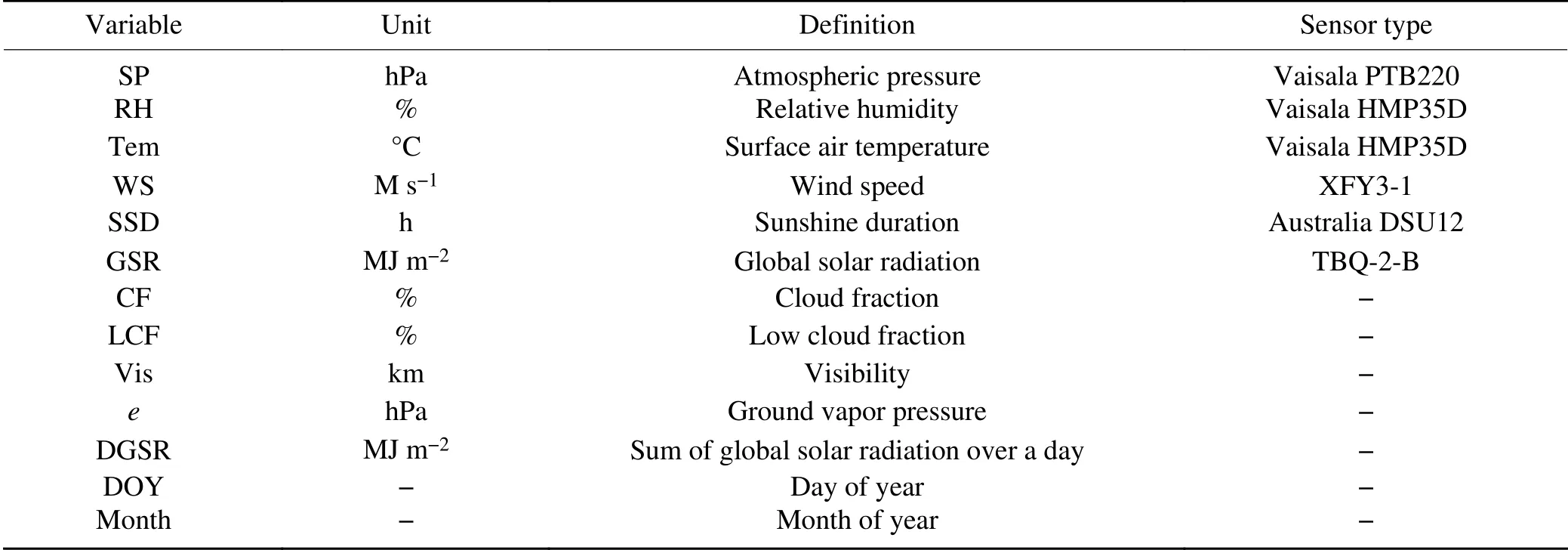
Table 1.The short name,definition,and sensor type (if applicable) for each variable.

Fig.1.(a) Map showing the location of Zhongshan Station,(b) image of Zhongshan Station area,and (c) the solar radiation instrument in the meteorological observation field.
Solar radiation observations started relatively late(March 2008) at Zhongshan Station,although short-term observations and research projects of solar radiation were performed during the periods of January–February 1990 (Wang and Xiong,1991
) and February 1993 to December 1994(Bian et al.,1998
).The solar radiation dataset for 2008 to 2020 was first used in this study.The observation site is located in the meteorological field north of the station (as shown inFig.1b
),where the surface is exposed rock from November to February,and there is snow for a short time in other periods,although there is usually almost no snow.A TBQ-2-B pyranometer made by Beijing Huatron company(Fig.1c
) was used to measure global solar radiation with a wavelength range of 0.3 to 3 μm and a resolution of hours at this station.The measured signal range of the TBQ-2-B pyranometer is 0–2000 W m,the output signal is 0–20 mV,and the annual stability is ±2%.To ensure the accuracy of observation data,the TBQ-2-B pyranometer passed the verification and calibration of the China Meteorological Administration before installation.2.2.Model development
2.2.1.Data processing and time matching
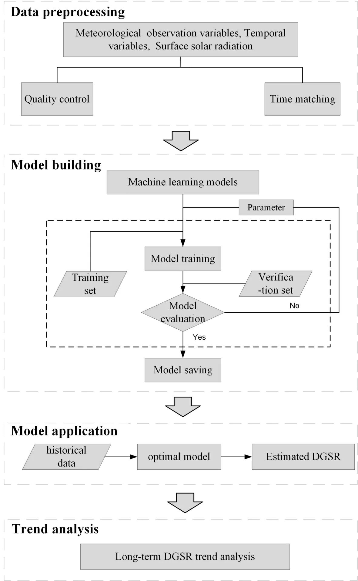
Fig.2.Steps of historical estimation and long-term trend analysis of DGSR at Zhongshan Station,Antarctica.
The meteorological observation data with a data quality code of 0 (passing all quality control checks) were extracted and time matched.The meteorological data observed at 0000,0600,1200,and 1800 UTC each day were then averaged to obtain the daily mean values.The DGSR and SSD were obtained as the sums of 24 hours per day.The final available data include conventional meteorological data from March 1989 to March 2020 and radiation observations from March 2008 to March 2020.Figure 3
shows the statistical properties (minimum,maximum,mean,and standard deviation) of the variables used for model training,testing,and hindcast estimation at Zhongshan Station during 2010–20.The DGSR (SSD) ranges from 0 (0) to 36.27 MJ m(21.70 hours),and the annual average value is 10.04 MJ m(4.83 hours).The annual average SP,Tem,RH,and WS are 985.08 hPa,−10.16°C,56.90%,and 6.49 m s,respectively.2.2.2.Model building
We evaluated the performances of multiple machine learning models for estimating DGSR at Zhongshan Station,including the RF (Chen et al.,2018
),Light Gradient Boosting Machine (LightGBM) (Ke et al.,2017
;Chen et al.,2019
),decision tree (DT) (Quinlan,1986
),back propagation neural network (BPNN) (Wen et al.,2002
),eXtreme Gradient Boosting (XGBoost) (Zelterman,2015
),support vector machine (SVM) (Cortes and Vapnik,1995
),multiple linear regression (MLR) (Zelterman,2015
),and Adaptive Boosting (AdaBoost) (Wang,2012
) models.The RF model is a widely used machine learning model that has a highly flexible algorithm and the capacity to analyze complex interactions of data classifications with noise or missing values(Chen et al.,2018
).The RF model has also been used as a variable selection tool to select the input variables for a final model (Zeng et al.,2020
).The RF model uses a bagging method to produce the training dataset.The out-of-the-bag(out-of-bag,OOB) data were used to evaluate the veracity of the regression predicted by the RF model.OOB estimation was an unbiased estimation when the number of trees was sufficient.In common statistical methods,overfitting occurs frequently when the methods have high degrees of freedom.In contrast to other models (e.g.,the BPNN and SVM models),the RF model is an ensemble of random trees and basically has no issue of overfitting.LightGBM is a gradient promotion framework based on decision trees and can model complex nonlinear functions.LightGBM has the advantages of distributed and high performance in sorting,classification,and regression (Chen et al.,2019
).The DT is a common and extensively researched solution to classification and prediction (Quinlan,1986
).The BPNN is a multilayer feedforward neural network based on a mathematical technique named Bayesian regularization to convert nonlinear regression into “well-posed” problems (Wen et al.,2002
).The BPNN is composed of three layers:an input layer (first layer),hidden layer (middle layer),and output layer (last layer).XGBoost is a boosting algorithm with high performance for various regression and classification issues.The XGBoost method requires less training and time for prediction and can improve computing speed and accuracy (Gui et al.,2020
).The SVM was developed by Vapnik-Chervonenkis dimension theory and structural analysis of the minimum risk principle.The SVM exhibits a unique advantage in dealing with small-sample problems,nonlinear cases,and high-dimensional pattern recognition problems by its kernel functions (Cortes and Vapnik,1995
).MLR is the regression analysis involving two or more independent variables.The MLR model can intuitively and quickly analyze correlations between multiple variables and dependent variables (Zelterman,2015
).Hence,MLR has been widely used in social science,economics,and technology.AdaBoost is an excellent boosting algorithm that combines multiple weak classifiers into a strong classifier.The main purpose of AdaBoost is to train different learning devices on the same training set and then combine these devices to construct a stronger final learning device (Wang,2012
).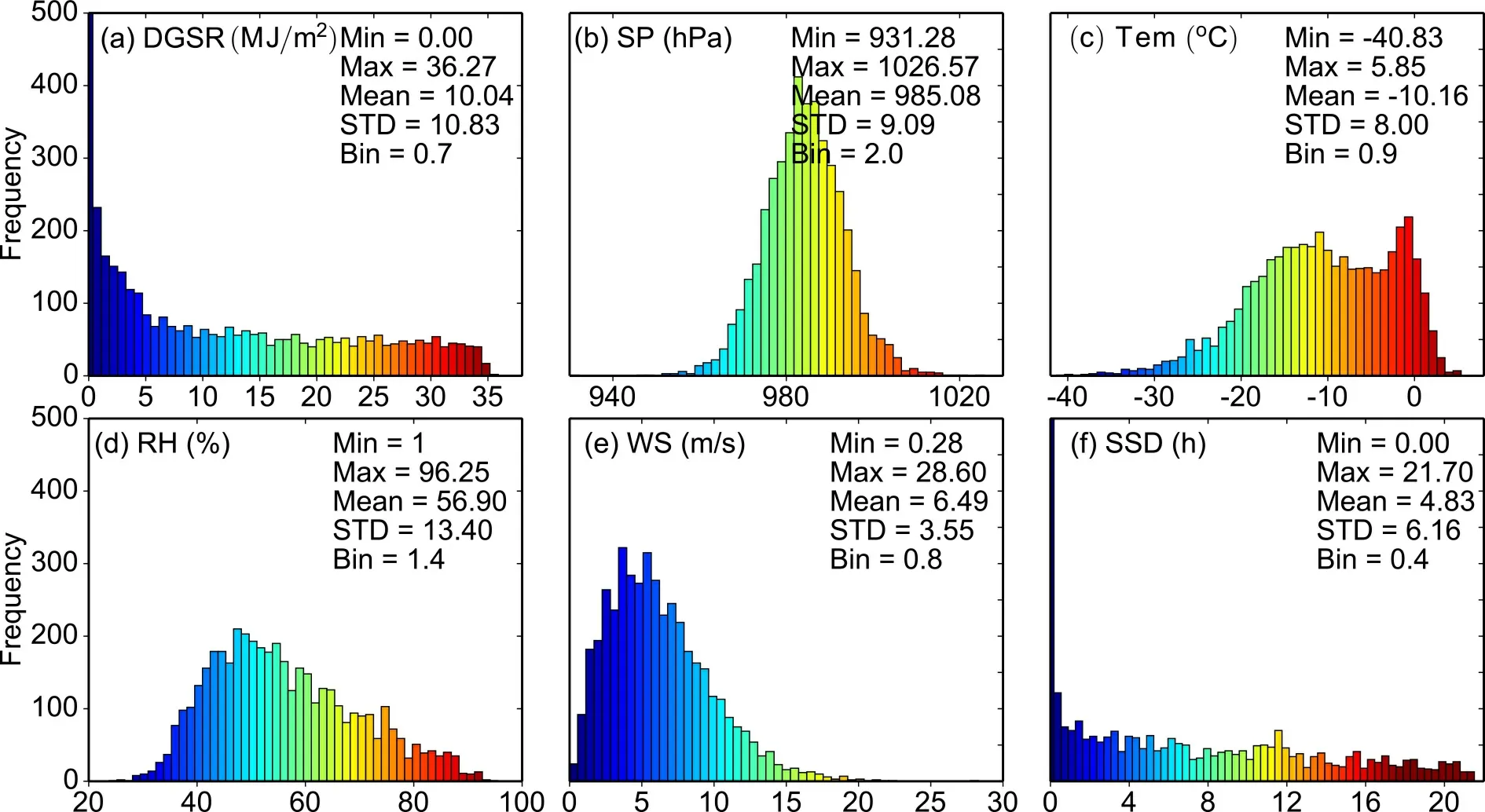
Fig.3.The frequency distribution of (a) observed DGSR,(b) SP,(c) Tem,(d) RH,(e) WS,and (f) SSD at Zhongshan Station,Antarctica during 2010–20 for model training and cross-validation.
The model with the best estimated performance will be the final model in this study.As in previous work (Zeng et al.,2020
),to obtain the optimal machine learning model,the results of 10-fold cross-validation (10-fold CV) were used to evaluate the model performances with different parameters (the final parameters of the models are shown inTable 2
).In 10-fold CV,the matched pairs were partitioned into ten parts in equal proportion,with the first part as the testing subset and the other nine parts as the training subsets.This step was repeated ten times until every subset was tested,and the estimation results (mainly consisting of the coefficient of determination,R,root-mean-square error,RMSE,and mean absolute error,MAE) of the 10 parts were averaged and used as the accuracy of the final model.The accuracy indicators,including the R,RMSE,MAE,and difference (estimated minus observed),were used to assess the capabilities of the machine learning models and then obtain an optimal model (Gui et al.,2020
;Zeng et al.,2020
).In this study,we used the data from April 2010 to March 2020 for training,the 10-fold CV method for testing,and the period from April 2008 to March 2010 for evaluating the historic estimates.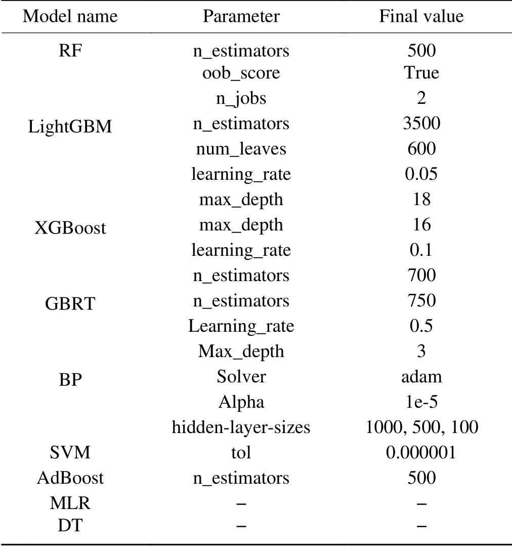
Table 2.The final selected values of the main parameters for each model.
2.2.3.Model application
The optimal model obtained from the above modelswas applied to estimate the DGSR using meteorological measurements recorded at Zhongshan Station from March 1989 to February 2020.The time variations in DGSR estimated by the optimal model were then compared with the observed DGSR.Finally,the long-term historical estimated DGSR at Zhongshan Station was analyzed,and then changes in the trend and the possible factors influencing these changes were further investigated.
2.3.Methods for DGSR trend analysis
Least squares regression has been applied to detect the linear trend in DGSR annual anomalies (Guo et al.,2017
).Five-year running means of DGSR anomalies have been used to visually display the DGSR trend (Xue et al.,2019
).In addition,the sliding trend analysis method has been used to help examine the time nodes of changes because trends often change with the span of the variable calculation period(Che et al.,2019
;Gui et al.,2019
).According to the method fromGui et al.(2019)
,we used Student’s t tests to detect the robustness of each trend,and the criterion for statistical significance was set at the 95% confidence level.Since the estimated DGSR dataset and meteorological observation dataset have complete records of the whole year for each year from 1990 to 2019,the study period is set as 1990–2019 for the analyses of the monthly variations in meteorological variables and DGSR and the long-term changes in the DGSR trend.3.Results and discussion
3.1.Validation and comparison of models
Figures 4a
and4b
show the scatterplots of the fitted model and 10-fold CV model results of the RF model from April 2010 to March 2020 at Zhongshan Station,Antarctica.Compared with those of other models,we found that the fitted and 10-fold CV results of the RF model have higher Rvalues of 0.997 and 0.988 and lower RMSE (MAE) values of 0.547 (1.189) MJ mand 0.278 (0.648) MJ m,respectively.To assess the performance of the hindcast estimated by the RF model,the hindcast estimated results from April 2008 to March 2010 are shown inFig.4c
.We found that the hindcast estimated DGSR presented good consistency with the observed DGSR (R=0.984,RMSE=1.377 MJ m,and MAE=0.828 MJ m).To further examine the hindcast performance of the DGSR estimated by the RF model,as an example,we selected historical estimated DGSR in 2009 (obtained from hindcast estimated results during April 2008 to March 2010) for comparison with the ground observed DGSR.Figure 5a
shows the daily time series (Fig.5b
depicts the difference) of observed DGSR and estimated DGSR at Zhongshan Station.These two time series are highly consistent with each other,and the higher daily(monthly) mean difference values mainly occur in the summer,especially in the polar day period,but do not exceed±5 (±0.85) MJ m.Figure 5b
also shows that approximately 96.7% (343 days in 2009) of the difference values(observed DGSR minus estimated DGSR) fell within the range of ±2 MJ m.The results indicate that the DGSR estimated by the RF model closely fits the observed DGSR.Considering the CV results and the accuracy of the historic estimates,the RF model is highly recommended for DGSR estimation at Zhongshan Station in this study.The relative importance of the variables in the RF model is illustrated in Fig.S1 in the electronic supplementary material (ESM).As shown in Fig.S1,SSD plays a dominant role in terms of the relative importance in the RF model and accounts for 60.3%of the overall importance.This result is consistent with previous studies showing that SSD is significantly correlated with DGSR (Wang et al.,2016
;Zeng et al.,2020
).The results also indicate two other dominant variables:DOY and Tem (accounting for 16.8% and 16.1% of the overall importance,respectively).These results suggest that DOY (seasonal effects) and Tem are also critical for DGSR estimation.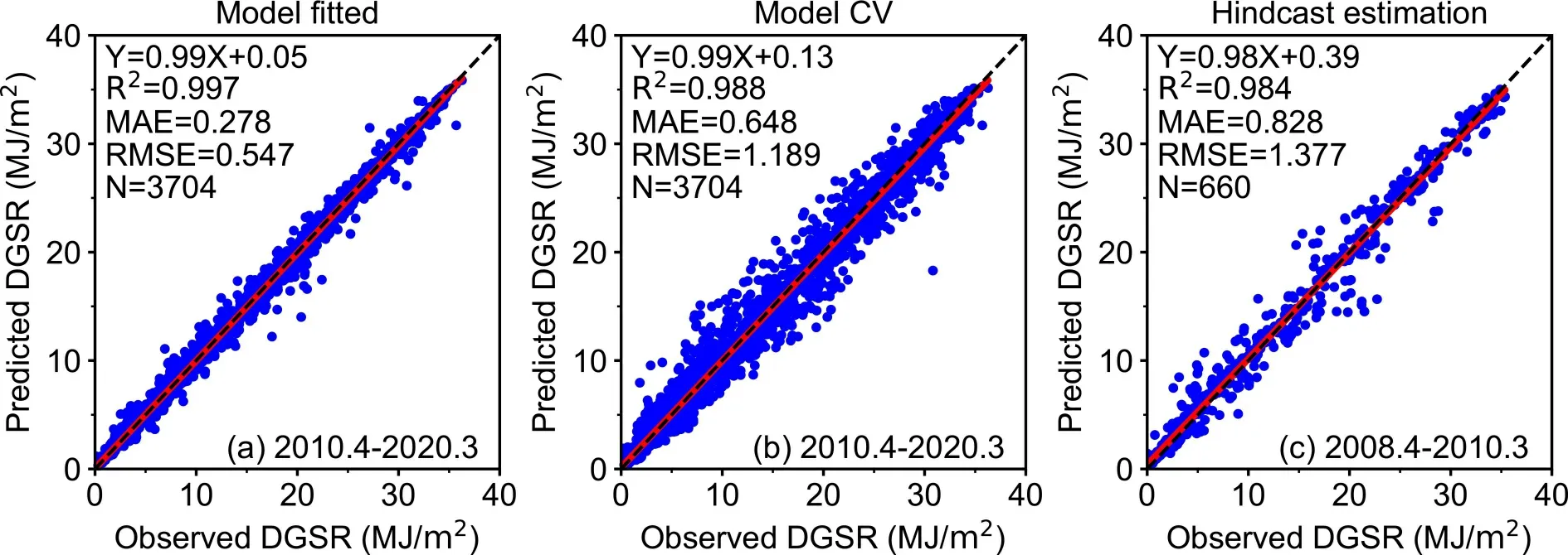
Fig.4.Scatterplots of the (a) fitted model,(b) CV model,and (c) hindcast estimation results of the RF model at Zhongshan Station,Antarctica.
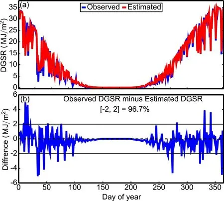
Fig.5.The (a) time series of observed (blue) versus estimated(red) DGSR and the (b) corresponding difference (observed DGSR minus estimated DGSR) in 2009 at Zhongshan Station,Antarctica.[−2,2] indicates a difference within ±2 MJ m−2.
In addition to evaluating the performance of the RF model,we also evaluated the performances of other commonly used machine learning models for estimating DGSR at Zhongshan Station.From the results of the performance comparison inTable 3
,the RF model performs better than the other models,and the LightGBM,XGBoost,BPNN,and gradient boosted regression tree (GBRT) models show similar historic estimation abilities,followed by those of the DT and AdBoost models.The SVM and MLR models have the worst performances.In common statistical methods,overfitting frequently occurs when the methods have highdegrees of freedom.In contrast to other models,the RF model is an ensemble of random trees and has no issue of overfitting in this study.
Table 3.The results of the fitted model,10-fold CV model,and historical estimation power by different machine learning models.
Overall,these comprehensive results further confirm that the RF model has reliable performance in estimating historical DGSR.We can expect that it will be feasible to reconstruct the historical DGSR based on meteorological observation data and the RF model.Thus,the estimated historical dataset is used to accurately describe the comprehensive characteristics and changes in the long-term trend of DGSR.Therefore,we mainly use the DGSR estimated by the RF model for 1989 to 2020 in the following trend analysis.
3.2.Monthly and annual variations in DGSR
Before analyzing the changes in the DGSR trend,we calculated the monthly and annual characteristics of DGSR estimated by the RF model and the corresponding meteorological variables over the period of 1990–2019 (as shown inFig.6
).The estimated DGSR shows significant monthly and seasonal changes,in which the DGSR during the halfyear of summer (October to March) is significantly higher than that during the half-year of winter (April to September),and the higher DGSR values,up to 30 MJ m,are mainly during the polar day period,while the DGSR values are 0 MJ mduring the polar night period.The monthly average humidity varies from 56% to 61% from 1990 to 2019 and is higher in summer than in other seasons.The monthly mean temperature varies from −2.90°C to 0.24°C in summer and from −14.74°C to −16.12°C in winter.The monthly average temperature is the highest in January (0.24°C) and the lowest in July (−16.18°C).Variations in surface pressure at Zhongshan Station are characterized by half-year waves.From January to June,there are periods of high pressure,and other months have periods of low pressure.The highest (lowest) monthly average surface pressure occurs in June (October) and is greater than 988 hPa (lower than 981 hPa).The wind speed is the highest in winter,followed by that in autumn,spring,and summer.The highest (lowest) monthly average wind speed is 7.94 m s(5.01 m s) in August (January).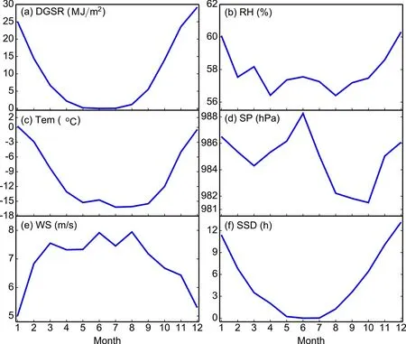
Fig.6.The monthly variation in (a) DGSR (estimated),(b) SP,(c) Tem,(d) RH,(e) WS,and (f) SSD at Zhongshan Station,Antarctica during 1990–2019.
Zhongshan Station is located on the edge of the Antarctic continent and is near the Antarctic ice sheet.The winds at this station are mainly affected by a combination of the easterly airflow in the northern part of the Antarctic continent,polar cyclones,and katabatic winds.Easterly winds prevail over this station year-round.In summer (December,January,and February),both the Antarctic continental cold highpressure system and the circumpolar low-pressure zone are weaker,and the smaller pressure gradient between these two synoptic systems induces a lower wind speed.In winter(April,May,and June),the prevailing Antarctic continental high-pressure system strengthens,and the circumpolar lowpressure zone moves southward,which causes a larger pressure gradient and thus results in a higher wind speed.Additionally,the monthly variations in air pressure at Zhongshan Station are closely related to these two synoptic systems.Zhongshan Station is covered by snow and ice and the air has lower relative humidity in winter,while the snow and sea ice around this station melt in summer and thus cause increased saturation of water vapor in the air and higher relative humidity.It is noted that the long sunshine duration and strong solar radiation in summer play key roles in the temperature increase at this station.
The monthly variation in SSD is basically consistent with that in DGSR,and the Rbetween SSD and DGSR is 0.88,indicating that SSD is the main input variable for DGSR in the machine learning models.Figures S2 and S3 in the ESM show that the yearly average value of the estimated DGSR coincides with that of the measured DGSR from 2009 to 2019 (and also in 1994),and the differences (estimated DGSR minus observed DGSR) were mainly distributed between −0.1 and 0.1 MJ m.Furthermore,the annual changes in the estimated DGSR and observed SSD trends are highly consistent,suggesting that historical DGSR estimated by the RF model has high accuracy for further analysis(such as annual anomaly trends and sliding trends).
3.3.DGSR trend
Note there is continuous presence and absence of solar radiation at Zhongshan Station during summer and winter,respectively,because Antarctica experiences the peculiar conditions of polar day (beginning on 23 November and ending on 21 January of the following year at this station) and polar night (beginning on 27 May and ending on 18 July each year at this station).In addition,the DGSR values are 0 MJ mduring the polar night period.Therefore,the DGSR trend analysis was divided into the following three scenarios:all days of the year (annual,scenario 1),the polar day period (scenario 2),and the period of all days of the year except for polar day and polar night (scenario 3).Figures 7a
–7c
show the DGSR anomalies and their trends for the three scenarios.It can be seen that the trend of the DGSR annual anomalies increases during 1990–2004 and then begins to decrease after 2004.However,obvious differences in anomaly values exist among the three scenarios.The variation in DGSR anomalies is the greatest during the polar day period (increasing linear trend of 0.175 (MJ m)yrand decreasing linear trend of −0.101 (MJ m) yr,which are significant at the 95% confidence level),followed by that during all days of the year (increasing linear trend of 0.039 (MJ m) yrand decreasing linear trend of−0.025 (MJ m) yr,which are significant at the 95% confidence level),and it is lowest during the period of all days of the year except for polar day and polar night (increasing linear trend of 0.011 (MJ m) yrand decreasing linear trend of −0.001 (MJ m) yr,which are not statistically significant).In general,the trend of DGSR is similar to Europe(except for China,with a decreasing trend between 1990 and 2000) during the period of brightening,increasing slightly to early 2005,after which it shows a decrease to the present (Che et al.,2005
;Ohmura,2009
).At the Zhongshan Station,the Earth’s surface receives more solar radiation during the polar day period because the sun always stays above the horizon.From 1990 to 2019,the average DGSR during the polar day period varies between 26 MJ mand 31 MJ m.However,the annual average DGSR varies from 9.6 MJ mto 10.8 MJ m.Therefore,the anomaly values and the range of variation during the polar day period are higher than those during all days of the year.The anomaly values during the period of all days of the year except for polar day and polar night alternate between positive and negative,indicating that the change in total solar radiation during this period basically has no obvious trend.The maximum value of the annual anomalies occurs during approximately 2004/05 and is mainly related to the days with precipitation (such as snowfall,which can result in low visibility and then decreased sunshine duration and solar radiation) at Zhongshan Station in Antarctica.In contrast to scenario 3 (all days of the year except for polar day and polar night),scenario 2 (the polar day period) and scenario 1 (annual) have similar trends in the anomalies(and the sunshine duration during the polar day period accounts for approximately 45% of the total sunshine duration of each year),indicating that the changes in sunshine duration and DGSR during the polar day period play a leading role in the changes in the trend of the DGSR annual anomalies.
Based on Student’s t tests,the sliding trends of DGSR for all situations are shown inFigs.7d
–7f
to present a more comprehensive analysis of the annual trends.Sliding trends are calculated for the three scenarios,starting in each year from 1990 to 2015 and ending in 2019 with increments of at least five years.As shown in scenario 1 (all days of the year),the trend of DGSR increases from 1990 to 2003(although an opposite trend is found during approximately 1993 and 1995),then declines sharply after 2004 (especially in scenario 2:the polar day period),and slightly increases in 2012.The sliding trends for scenario 3 (all days of the year except for polar day and polar night) are smaller and relatively stable compared with those for the other scenarios.When the running mean window is longer than 15 years,the DGSR trends first increase and then decrease in scenario 3 (all days of the year except for polar day and polar night),and most of the trends are statistically significant.3.4.The potential impact factors of DGSR
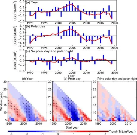
Fig.7.Time series of the annual mean anomalies of estimated DGSR:(a) annual mean but no polar night,(b) polar day,and (c) no polar day and no polar night.The red lines indicate the 5-year running means of the DGSR anomalies.Sliding-window trend analyses of annual mean estimated DGSR at Zhongshan Station,Antarctica,from 1990 to 2019 for (d) all years but no polar night,(e) polar day,and (f) no polar day and no polar night.
DGSR is affected by cloud cover,water vapor,and aerosols before reaching the surface (Che et al.,2005
).However,aerosols are relatively low over the Antarctic,so they will not be discussed in this study.In contrast,bad weather events (fog,snowfall,blowing snow,and snowstorms) with low visibility are frequent at Antarctic Zhongshan Station and also affect DGSR.Therefore,the effects of cloud fraction,low cloud fraction,ground vapor pressure (e,which represents atmospheric water vapor content),and visibility (which represents bad weather events)on DGSR at this station are further detailed and explicitly analyzed.Note that solar radiation is greatly affected by solar altitude angle in the polar region (which experiences the phenomena of polar day and polar night).To avoid the effects of these phenomena and analyze the influence of potential factors on solar radiation,we selected only the matched samples of April and September each year for discussion in this study.Here,all the matched samples are divided into five subsets according to cloud cover (0%–20%,20%–40%,40%–60%,60%–80%,and 80%–100%),low cloud cover(0%–20%,20%–40%,40%–60%,60%–80%,and 80%–100%),and ground vapor pressure (0–1 hPa,1–2 hPa,2–3 hPa,3–4 hPa,and >4 hPa),and then the average DGSR is calculated for each subset and the results are shown inFigs.8a
,8b
,and8c
,respectively.Similarly,the matched samples are divided into six subsets according to visibility(0–5 km,5–10 km,10–15 km,15–20 km,20–25 km,and>25 km),then the average DGSR is calculated for each subset (results shown inFig.8d
).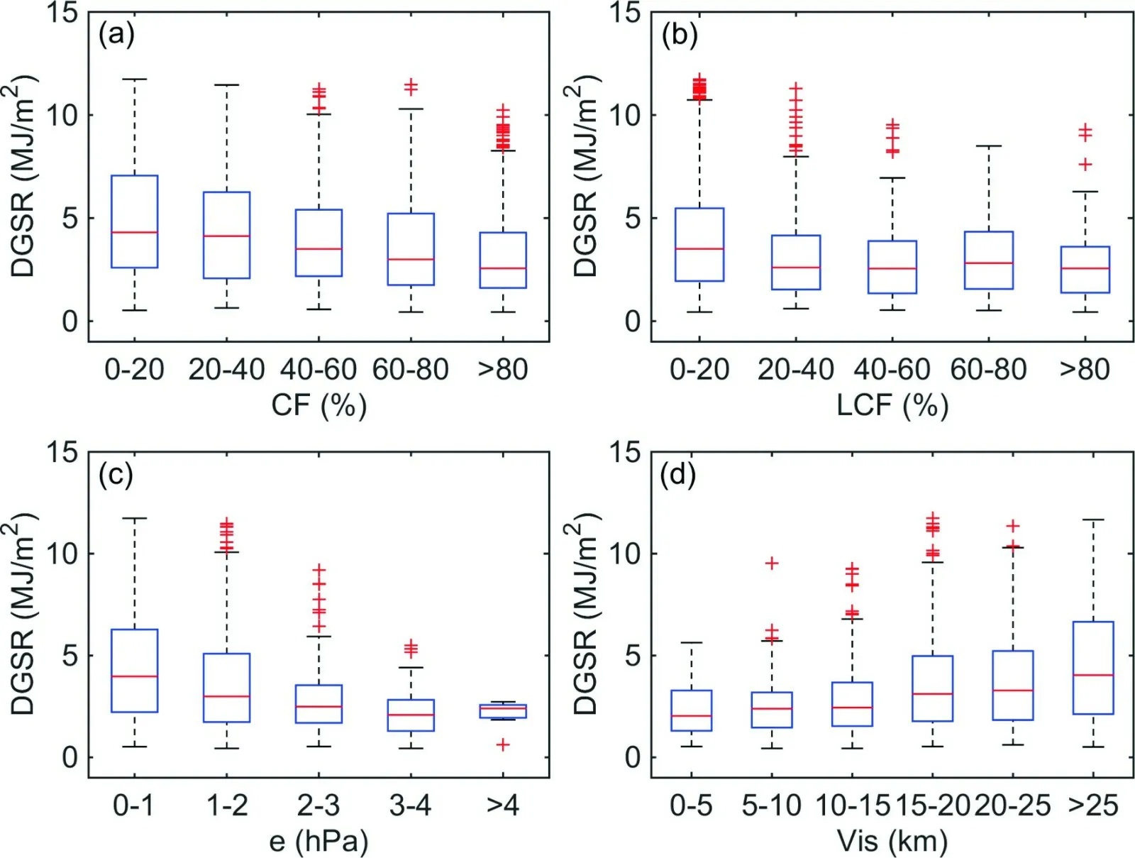
Fig.8.The effect on the estimated DGSR by the different (a) CF,(b) LCF,(c) e,and (d) Vis conditions at Zhongshan Station,Antarctica.
We found that DGSR significantly decreases (significantly increases) with increasing cloud fraction and ground vapor pressure (visibility).This is because under cloudy conditions,solar radiation reflects back to the top of the atmosphere,reducing the amount of solar radiation reaching the Earth’s surface.However,DGSR does not change much when the low cloud fraction is greater than 40%.We also found that DGSR is generally low during severe weather with low visibility but is significantly higher under high visibility conditions.Overall,DGSR decreases with increasing cloud cover,low cloud cover,and ground vapor pressure but increases with increasing visibility.The change in DGSR with low cloud cover is not significant with the change in cloud cover,ground vapor pressure,and visibility.Meanwhile,the time series of DGSR,LCF,CF,e,Vis,and SSD and their long-term trends are examined in Figs.S4a–S4f,respectively.DGSR shows a small upward trend.Accordingly,SSD and Vis exhibit upward trends (CF,LCF,and e exhibit downward trends),implying that the cloud cover,water vapor,and abnormal weather (except as solar altitude angle in the polar region) are the common factors that influence the trend of DGSR at this station.To sum up,clouds and water vapor in the atmosphere are the main factors affecting solar radiation.Bad weather conditions,such as fog,blowing snow,and snowstorms,are also a major factor affecting solar radiation at Zhongshan Station,Antarctica.
4.Concluding remarks
Based on ground meteorological observation data,an RF model was developed to estimate DGSR,and a high-precision,long-term DGSR dataset was constructed for 1989 to 2020 at Zhongshan Station,Antarctica.Long-term trends and the potential impact factors of DGSR were then analyzed in this study.Compared with those of other models,we found that the fitted and 10-fold CV results of the RF model have higher Rvalues and lower RMSE and MAE,and the hindcast estimated DGSR presents good consistency with the observed DGSR (R=0.984,RMSE=1.377 MJ m,and MAE=0.828 MJ m).The RF model is better than other models for reconstructing the historical DGSR based on the meteorological observations in this study.The DGSR trends were very consistent in all situations,and DGSR generally increased during 1989–2004 and then began to decrease after 2004.The sliding trend of DGSR in the all days of the year except for polar night period and the polar day period increased from 1990 to 2003 (although an opposite trend was found during approximately 1993 and 1995 for the all days of the year except for polar night period),then declined sharply after 2004 and slightly increased in 2012,while the sliding trends for the period of all days of the year except for polar day and polar night were smaller and relatively stable.DGSR decreases with increasing cloud cover,low cloud cover,and ground vapor pressure but increases with increasing visibility.The results show that clouds and water vapor are the main factors affecting solar radiation in Antarctica.Meanwhile,bad weather conditions,such as fog,blowing snow,and snowstorms,are also a major factor affecting solar radiation at Zhongshan Station,Antarctica.Based on the DGSR estimation method in this study,our plan for future work can be divided into two parts:the first part is to construct a virtual DGSR observation network across the Antarctic region,and the second part is to reconstruct historical site-scale DGSR through this newly constructed virtual DGSR observation network.It is worth noting that some sites in remote areas of Antarctica lack DGSR datasets.Therefore,these high-precision,long-term DGSR datasets can be used to study the radiation balance and the ultimate source of solar energy in Antarctica.
:This work was supported by the National Natural Science Foundation of China (Grant Nos.41941010,41771064 and 41776195),the National Basic Research Program of China (Grant No.2016YFC1400303),and the Basic Fund of the Chinese Academy of Meteorological Sciences (Grant No.2018Z001).We greatly appreciate the help from the Polar Research Institute of China and the Antarctic expeditioners at the Chinese Zhongshan Station.The long-term (March 1989–February 2020) estimated DGSR dataset can be acquired in the Mendeley data repository (data identification number:http://dx.doi.org/10.17632/2y2mmhzvcx.1
).Supplementary material is available in the online version of this article athttps://doi.org/10.1007/s00376-021-0386-6
.杂志排行
Advances in Atmospheric Sciences的其它文章
- The First Global Carbon Dioxide Flux Map Derived from TanSat Measurements
- A Deep Learning Method for Bias Correction of ECMWF 24–240 h Forecasts
- A Positivity-preserving Conservative Semi-Lagrangian Multi-moment Global Transport Model on the Cubed Sphere
- Thinner Sea Ice Contribution to the Remarkable Polynya Formation North of Greenland in August 2018
- Application of Backward Nonlinear Local Lyapunov Exponent Method to Assessing the Relative Impacts of Initial Condition and Model Errors on Local Backward Predictability
- Variational Quality Control of Non-Gaussian Innovations in the GRAPES m3DVAR System:Mass Field Evaluation of Assimilation Experiments
