Variational Quality Control of Non-Gaussian Innovations in the GRAPES m3DVAR System:Mass Field Evaluation of Assimilation Experiments

Jie HE ,Xulin MA* ,Xuyang GE ,Juanjuan LIU ,Wei CHENG ,Man-Yau CHAN ,and Ziniu XIAO

1Collaborative Innovation Center on Forecast and Evaluation of Meteorological Disasters,Key Laboratory of Meteorological Disaster,Nanjing University of Information Science and Technology,Nanjing 210044,China

2State Key Laboratory of Numerical Modeling for Atmospheric Sciences and Geophysical Fluid Dynamics,Institute of Atmospheric Physics,Chinese Academy of Sciences,Beijing 100029,China

3Beijing Institute of Applied Meteorology,Beijing 100029,China

4Department of Meteorology and Atmospheric Science,and Center for Advanced Data Assimilation and Predictability Techniques,The Pennsylvania State University,University Park,PA 16801,USA

ABSTRACT The existence of outliers can seriously influence the analysis of variational data assimilation.Quality control allows us to effectively eliminate or absorb these outliers to produce better analysis fields.In particular,variational quality control(VarQC) can process gray zone outliers and is thus broadly used in variational data assimilation systems.In this study,governing equations are derived for two VarQC algorithms that utilize different contaminated Gaussian distributions(CGDs):Gaussian plus flat distribution and Huber norm distribution.As such,these VarQC algorithms can handle outliers that have non-Gaussian innovations.Then,these VarQC algorithms are implemented in the Global/Regional Assimilation and PrEdiction System (GRAPES) model-level three-dimensional variational data assimilation (m3DVAR) system.Tests using artificial observations indicate that the VarQC method using the Huber distribution has stronger robustness for including outliers to improve posterior analysis than the VarQC method using the Gaussian plus flat distribution.Furthermore,real observation experiments show that the distribution of observation analysis weights conform well with theory,indicating that the application of VarQC is effective in the GRAPES m3DVAR system.Subsequent case study and longperiod data assimilation experiments show that the spatial distribution and amplitude of the observation analysis weights are related to the analysis increments of the mass field (geopotential height and temperature).Compared to the control experiment,VarQC experiments have noticeably better posterior mass fields.Finally,the VarQC method using the Huber distribution is superior to the VarQC method using the Gaussian plus flat distribution,especially at the middle and lower levels.

Key words:variational quality control,non-Gaussian distribution,innovation,outlier,data assimilation

1.Introduction

Quality control (QC) of meteorological data plays a crucial role in the data assimilation (DA) of the numerical weather forecast (NWP) system.The term "quality control"refers to the process of comparing observational data against a specified reference (e.g.,the climatological mean,surrounding observation,model state) and then subjectively deciding whether to reject or correct erroneous data (

Kal-

nay,2003

).The quality of the observations directly affects the errors in the initial conditions,and hence the accuracy of numerical weather prediction.Therefore,for more accurate and effective use of observations,meteorologists have developed many quality control methods to screen and correct the observations (

Fiebrich et al.,2010

).Quality control methods essentially aim to reduce various initial condition errors in NWP.Observation errors and background errors play a key role in the establishment of variational data assimilation (VarDA).Most popular DA methods [e.g.,3DVAR (

Courtier et al.,1998

),4DVAR (

Rabier et al.,2000

;

Rawlins et al.,2007

),and ensemble Kalman filters (

Houtekamer and Mitchell,1998

)] are based on the assumption that the random errors in observation and background follow Gaussian distributions and that the random observation errors are independent of the background random errors.Observation errors also include systematic and rough errors (

Gandin,1988

).Observations with systematic errors are usually corrected by bias correction prior to their assimilation (

Dee and Uppala,2009

).The latter,also called gross errors,are non-meteorological errors caused by measurement equipment failure,calculation errors,and transmission or reception errors.Observations with gross errors are often treated as outliers.These outlying observations are generally removed in DA systems using conventional quality control (CQC) methods,such as the background quality check(BgQC:

Järvinen and Undén,1997

;

Cardinali et al.,2003

).These CQC methods typically assume that random errors follow Gaussian distributions.However,not all outliers are observations with gross errors (

Hampel,2001

).Observations without gross errors can sometimes be classified as an outlier simply because their random error distributions do not follow a Gaussian distribution (

Tavolato and Isaksen,2015

).For example,consider the situation where a forecasted thunderstorm is substantially displaced from the observed thunderstorm and that a wind observation was made in the gust front of the observed thunderstorm.Since the observation site is far from the forecasted thunderstorm,the related innovation (observation minus background) would be extreme.In this situation,CQC methods are likely to reject the wind observation.Therefore,rejecting such observations as an outlier may be suboptimal.In view of the potential impact of outliers on numerical forecasting,their quality control is critical (

Storto,2016

;

Duan et al.,2017

).There have been many studies on CQC,such as range checking,extreme value checking,consistency checking,complex quality control,static analysis,and statistical checking(

Gandin,1988

;

Collins and Gandin,1990

;

Gandin et al.,1993

;

Vickers and Mahrt,1997

;

Fiebrich et al.,2010

).Although these CQC methods have been implemented widely,there are several issues with CQC methods.First of all,the CQC methods process the observations before the DA and after the bias correction process.This means that CQC accepted (removed) observations will not be removed(assimilated) even if they are identified as deleterious(valid) observations during the iterative analysis procedures.The second issue with current CQC methods is that there is some ambiguity in selecting rejection thresholds.For example,the background quality check,which assumes the observation and background errors to be Gaussian distributions,rejects outliers if the magnitude of their innovations exceeds a rejection threshold.This rejection threshold is empirically determined.An overly small threshold likely eliminates valid observations,whereas an excessively high threshold likely includes problematic observations.The third issue with current CQC methods is that an accurate observation might be rejected by CQC,even though its large innovation is simply due to non-Gaussian errors(

Lorenc,1984

;

Purser,1984

).For instance,outliers without gross errors are often observed in meso-and micro-scale weather events,such as severe storms and tropical cyclones,but CQC sometimes identifies them as outliers with gross errors and removes them.This erroneous rejection wastes observations and leads to suboptimal initial conditions.A final issue with CQC is that thresholds differ for different observation types.These recognized inadequacies have catalyzed the development of variational quality control (VarQC:

Anderson and Järvinen,1999

;

Storto,2016

;

Duan et al.,2017

;

Ma et al.,2017

),which can mitigate said inadequacies.VarQC implemented in VarDA assumes that the errors of valid observations and usable observations (the VO,UO,see details in our companion paper) respectively follow Gaussian distributions and non-Gaussian distributions.Since we cannot distinguish between VO and UO prior to quality control,the observation errors are treated as though they are drawn from the sum of a Gaussian and a non-Gaussian distribution (i.e.,the observation errors are drawn from a contaminated Gaussian distribution,CGD).With this in mind,a new observational cost function for the VarQC method (

Ingleby and Lorenc,1993

) is then obtained using Bayesian probability theory(

Lorenc,1986

).In the VarQC method,the non-Gaussian innovation distribution comes from non-Gaussian observation errors,while the background error has a Gaussian distribution.Therefore,during the iterative optimization of the cost function,different weights can be iteratively assigned to observations with non-Gaussian error to improve analysis or mitigate the negative effects of outliers on the posterior analysis.The VarQC method can thus effectively absorb the usable information from these outliers during VarDA.The VarQC method of

Anderson and Järvinen (1999)

has been developed in the 3DVAR assimilation of the GRAPES (Global/Regional Assimilation and PrEdiction System) regional model in our prior work (

Ma et al.,2017

).Within it,VarQC was implemented with the Gaussian plus flat distribution for observation errors.The main goal of this study is to implement another VarQC method with Huber distribution (

Tavolato and Isaksen,2015

) in the GRAPES m3DVAR ("m" represents model level) system.The performance of the new system is demonstrated using the mass field(geopotential height and temperature).

In section 2,we will discuss the various VarQC schemes.We will also illustrate the non-Gaussian innovation distributions caused by non-Gaussian observation errors for different observation types using the assimilated data of the GRAPES model.The data and experimental design are described in section 3.Section 4 presents the idealized testing and the real-data experimental results of two VarQC methods.Finally,conclusions and discussions are shown in section 5.

2.VarQC with non-Gaussian innovations

2.1.VarQC with non-Gaussian observational error distribution mode

VarDA assumes that the independent errors from observation and background are Gaussian-distributed and that the probability of outliers (gross errors) is zero,implying all the outliers can be removed with the CQC strategy.However,not all outliers are a result of gross errors.Such outliers contain useful information and thus should not be removed(

Hampel,2001

).Moreover,with the imperfect CQC,the outliers probably occur in the assimilated observations due to the ambiguous rejection threshold.As a result,outliers that make it past the CQC results in innovation distributions with long,non-Gaussian tails (i.e.,the estimated innovation frequencies have a slower decay rate with larger innovations than the decay rate predicted by the Gaussian distribution,as seen in

Fig.1

).In this study,we will only consider the non-Gaussianity of observation errors caused by outliers.It is well-known that improving the consistency between the assumed observational error distribution mode (OEDM) and the actual mode can generate a more accurate posterior solution in DA(

Fowler and Van Leeuwen,2013

;

Legrand et al.,2016

).

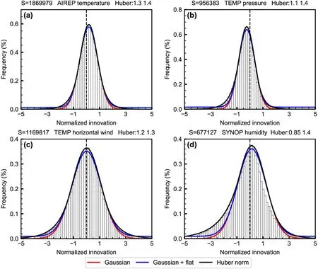
Fig.1.Statistics of innovations (normalized by observational error) for (a) aircraft-reported temperature,(b)radiosonde pressure,(c) radiosonde horizontal wind,and (d) surface humidity.The red,blue,and black lines are,respectively,the Gaussian,Gaussian plus flat,and Huber norm distributions that have been fitted to the histograms of normalized innovations.The titles of the panels also indicate the fitted left and right transition points for Huber distribution,as well as the observation sample size (S).The observations are obtained from the domain in Fig.2 from 1 July to 31 September 2013.

In order to obtain a better analysis,the contaminated Gaussian distribution (

Tukey,1960

) is put forward to reduce (absorb) the impacts (information) of outliers on the posterior analysis.Compared to the Gaussian distribution,the contaminated Gaussian distribution is a better OEDM.In general,the contaminated Gaussian distribution is written as the sum of a Gaussian distribution (the “main” distribution) and some other distribution (the “perturbation” distribution;e.g.,Gaussian distributions with different means and variances).The CGD is expressed mathematically as:

where ε is the contamination rate (the prior probability of outliers),N is the Gaussian “main” distribution,and H is the perturbation (contaminating) distribution.Compared to the Gaussian distribution,the CGD can better fit the long tails in the actual observation error distribution that is widely used to deal with outliers in the field of surveying and mapping(

Yang,1991

;

Zhu,1996

).One possible choice of the perturbation distribution in Eq.(1) is the flat distribution (box-car:

Lahoz and Schneider,2014

).When used as an OEDM,the Gaussian plus flat distribution is consistent with the long-tail observations,meaning that these observations can be used effectively.In contrast,these observations would have been removed during the gross check of CQC.Following Eq.(1),the Gaussian plus a flat distribution

P

is defined as

where F is the perturbed flat distribution (

Anderson and Järvinen,1999

).Using Eq.(2),we can derive an observational cost function (

J

) from applying the CGD into Bayes’ theorem.It is an updated cost function with respect to the old observational cost function [

J

=δ/2; see the statement of δ in Eq.(6)] under an assumption of Gaussian error distribution (N)in 3DVAR.We can subsequently derive the gradient function (∇

J

) and weight function (

W

) of variational quality control.These are shown below: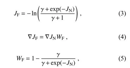

Apart from the flat distribution,the Laplace distribution can be used as the perturbation distribution.The Laplace distribution is used frequently as the perturbation distribution because it is a powerful tool in robust statistics(

Huber,2011

).The Gaussian plus Laplace distribution,a special CGD (

Huber,1972

;

Tavolato and Isaksen,2015

),is defined as

where the c is the transition value and δ is the normalized innovation [normalized using the observational standard deviation (σ);see also (

Tavolato and Isaksen,2015

)].Note that there are two transition points,−

c

(left transition point) and+

c

(right transition point),which are calculated by fitting the normalized innovation histograms.These transition point values are shown in the titles of the panels in

Fig.1

.This is similar to the search for transition point values described in

Tavolato and Isaksen (2015)

.The magnitude of both transition points is likely affected by the frequency of outliers.These outliers are generally frequent in extreme weather events.This Gaussian plus Laplace CGD is also known as the Huber norm distribution and is a commonly used OEDM in the field of robust statistics.The robustness of using a Huber distribution,which refers to the insensitivity of small differences between the actual and the assumed mode (

Zhu and Zeng,1999

),means the posterior analysis must be as close as possible to the normal solution calculated at the assumed OEDM (

Zhu,1996

).It is regularly used to respond to the impacts of outliers.With the Huber distribution in Eq.(6),we can derive the updated observational cost function (

J

),gradient function (∇

J

),and weight function (

W

) of VarQC with respect to that of

J

.They are as follows: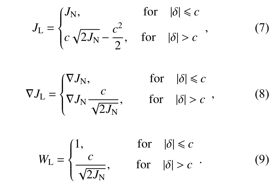

As seen in other fields,Huber distribution methods can yield more accurate and robust solutions than methods using Gaussian-distributed errors (

Guitton and Symes,2003

;

Huber,2011

).This increased robustness suggests that the use of the Huber distribution might be able to alleviate the negative impacts of outliers on the optimization analyses.Therefore,VarQC using the Huber distribution (hereafter referred to as “Huber-VarQC’’) can potentially produce more promising applications with respect to Flat-VarQC.

2.2.Non-Gaussian observational errors in the GRAPES m3DVAR

To illustrate the non-Gaussian observation error characteristics of commonly assimilated observations,we compared several types of observations against the GRAPES background to obtain innovation statistics.These observations are obtained from the Global Telecommunications System(GTS) and span a period from July 2013 to September 2013.The observation types are surface observations(SYNOP),radiosonde observations (TEMP),automated aircraft reports (AIREP),ship observations (SHIP),and satellite winds (SATOB).Before examining the innovation statistics,it should be noted in this study that we will assume that the non-Gaussianity of the innovations are only due to non-Gaussian observation errors.For instance,if the innovation statistics follow a Gaussian plus flat CGD,then the observation errors follow a similar CGD.With this in mind,the transition points of the observation error Huber distribution can be determined by the innovation Huber distribution.

Figure 1

shows the result of fitting several distributions (Gaussian,Gaussian plus flat,and Huber norm) to the estimated innovation distribution for several variables for several observation types.It can be seen that near the center of the innovation histogram,the innovations for the AIREP temperature (

Fig.1a

) and TEMP pressure and wind (

Figs.1b

and

c

) are consistent with all three distributions.However,towards the tails of the innovation histogram,the Gaussian plus flat distribution and the Huber distribution are more consistent with the histogram than that of the Gaussian distribution.Furthermore,the Huber distribution best fits the long tails of the innovation statistics in

Fig.1

.Similar long tail and fitting characteristics have also been identified for the innovation statistics of other observed variables of the various observation types (temperature,pressure,and wind;not shown),except for specific humidity.In other words,the CGD better fits the innovation statistics of pressure,temperature,and wind observations.However,the distribution of specific humidity innovations cannot be reasonably fitted by any of the three profiles (

Fig.1d

).A similar issue with the humidity has been described by

Pires et al.(2010)

and

Tavolato and Isaksen(2015)

.Although the left tail is fitted reasonably by the Huber distribution,the left transition point of 0.85 implies that the contamination rate (～20%) is unreasonable.A reasonably normal contamination rate would be less than 10% for conventional observations (

Hampel,1977

).A detailed discussion of VarQC parameters can be found in our companion paper.

3.Experimental design

3.1.Model configurations

The new-generation operational numerical forecast system of the China Meteorological Administration,the GRAPES (

Chen et al.,2008

;

Zhang and Shen,2008

;

Ma et

al.,2009

;

He et al.,2019a

) model version 3.0,and its threedimensional variational assimilation system has been applied in modeling many weather phenomena.These phenomena include extreme weather events,typhoons,sandstorms,and floods (

Xu et al.,2012

;

An et al.,2016

;

Wang et al.,2016

).We have implemented two VarQC methods(Flat-VarQC and Huber-VarQC) within the GRAPES m3DVAR system.Here,we discuss these model confiurations,and we will examine the posterior analysis of the mass fields from these VarQC methods in section 4.

Figure 2

shows the domain used in the simulation experiments.The simulation domain is defined by a 351 × 251 grid in the horizontal,with a meridional and zonal spacing of 20 km.In the vertical,the domain is broken into 31 levels,with a model top pressure of 10 hPa.The operational forecasts from the Global Forecast System (GFS) are used to construct the initial and lateral boundary conditions(ICs and LBCs) used for running the GRAPES model.We have selected a region over east China (domain shaded in red in

Fig.2

) for validation of the VarQC methods established in this paper.This region was selected because the high terrain over west China,particularly over the Tibetan Plateau,induces complex thermodynamic and dynamical effects (

Wang and Zeng,2012

;

Bao and Zhang,2013

;

He et al.,2019b

) that make it difficult to obtain accurate simulations.

3.2.Idealized experiments

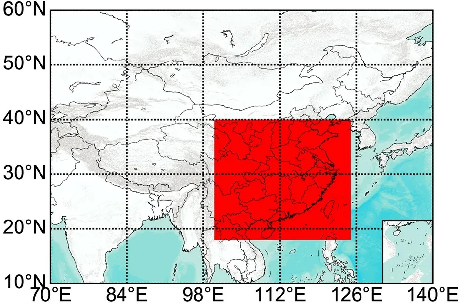
Fig.2.Simulation domain (10°−60°N,70°−140°E) used in running the GRAPES model for the real-data experiments of VarQC methods.The red shade shows the verified domain(18°−40°N,100°−125°E).

Both idealized and real-data experiments are performed.

Tables 1

and

2

describe the configurations of the idealized experiments used to examine the robustness of using the different VarQC methods to handle the outliers.The CTRL1 control experiment assimilates the actual pressure observations of 12 sounding sites,which are referred to as “normal pressures”.Some of these 500-hPa and 850-hPa level normal pressure observations are then replaced with outlier pressure values (underlined in

Table 1

).We will refer to these replaced observations as “outlier pressures” observations.Any pressure not equal to a specified level’s pressure will be treated as an outlier.For example,if an observed pressure at the 500-hPa height is not equal to 500 hPa,then that observation is an outlier.These outliers centered at the specified level are created by adding/subtracting a random draw from a uniform distribution within [1,2].The pressure errors (

Table 1

) from the observation report at 500 hPa(0.7766),850 hPa (0.7975),and other levels (not shown) are consistent in the idealized experiments.We examine the impact of assimilating these outlier pressures with/without VarQC using the experiments given in

Table 2

and detailed in section 4.1.The CTRL1 and CTRL1-Outlier experiments do not utilize any VarQC algorithms,whereas the Flat-Outlier and Huber-Outlier experiments respectively utilize the Flat-VarQC and Huber-VarQC methods.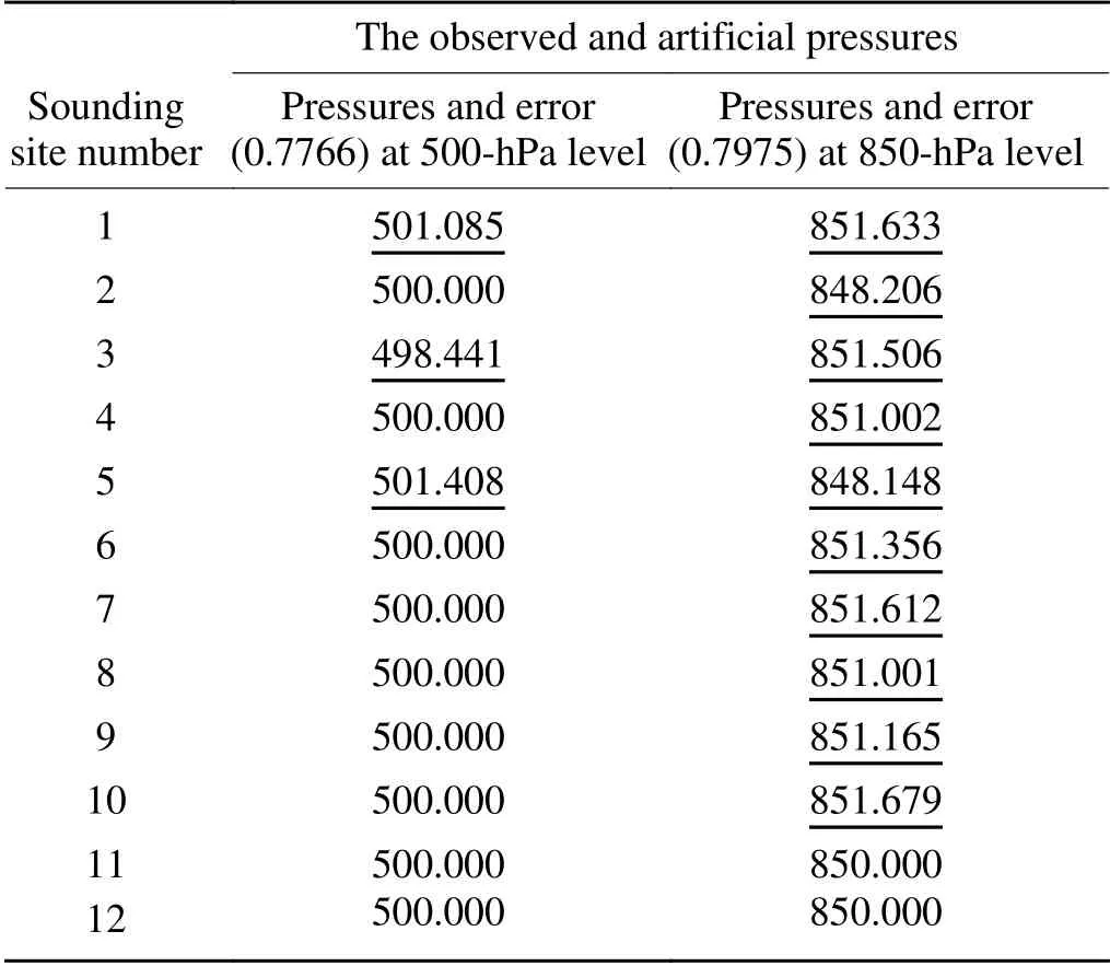

Table 1.The rebuilding outliers (underlined) for pressure (units:hPa) on sounding sites.

Table 2.Summary of the idealized experiment for different variational quality control.

Out of the 12 assimilated sounding sites,10 sites are scattered around East China,near the middle and lower reaches of the Yangtze River (

Fig.3a

).The remaining two sounding sites are located on the Korean Peninsula.Considering that observations that are sufficiently close can be used for "buddy checks" (

Auligné,2014

) during VarQC,the observations of sites 11 and 12 were not constructed as outliers(

Table 1

) since they are far from the other 10 sites.The pressure values from sites 1,3,and 5 at the 500-hPa level,as well as the pressure values from sites 1 to 10 at the 850-hPa level,were constructed as outliers (

Table 1

).Note that the pressures set as outliers would not be rejected by CQC.In other words,these outliers would be assimilated in all experiments,except for the CTRL1 experiment.Apart from CTRL1,which assimilates the normal pressures from 12 sounding sites without using VarQC,the other three experiments assimilate the same outlier pressures by using different quality control methods.

3.3.Real-data experiments

The configurations of the three real-data VarQC assimilation experiments are listed in

Table 3

.These experiments spanned the entire month of August in 2015 by using the fitted transition points from the training observations in 2013.Unlike the earlier idealized experiments,which only assimilated pressure observations,these real data experiments assimilated GTS observations.The GTS observation types include TEMP,SYNOP,AIREP,SHIP,and SATOB,and are assimilated using a 6-hour assimilation window into the three experiments.Furthermore,all three experiments are performed using the cold start method.The analyses are performed each day at 0000,0600,1200,and 1800 UTC.The experiments utilize the old BgQC threshold limit to evaluate the impacts of existing long-tails observations (identified in

Fig.1

).In this study,the Flat-VarQC was turned on during the first iteration of the 3DVAR cost function optimization in every cycle of the assimilation experiments.This first-iteration activation is unlike earlier work where VarQC’s modification to the 3DVAR cost function was only introduced after iterating the cost function minimization a specified number of times (

Anderson and Järvinen,1999

).This late-inclusion in earlier work was done to prevent convergence issues.We were able to activate the Flat-VarQC algorithm in the first iteration because we did not experience convergence issues in most cases.The only time where we experienced convergence issues is represented in

Fig.8b

.We were able to mostly avoid convergence issues because the first iterations’innovations were relatively small,meaning that the starting point of the Flat-VarQC-modified cost function minimization should be within or near the convex region containing the cost function’s global minima.Future work can investigate whether we should turn on the Flat-VarQC at a later iteration step.It should be noted that for the real-data experiments listed in

Table 3

,the innovations of specific humidity in the Huber-VarQC experiment cannot be effectively fitted by a Gaussian plus flat or a Huber norm OEDM in the statistics due to its unknown non-Gaussian property (

Pires et al.,2010

).To reduce the possibility of the Huber-VarQC experiment producing analyses that are worse than the CTRL2 experiment,while keeping VarQC active for specific humidity,we opted to use the OEDM that is closer to the traditionally prescribed Gaussian observation error distribution:the Gaussian plus flat OEDM.Thus,specific humidity observations in the Huber-VarQC are assimilated using the Gaussian plus flat OEDM,while all other observations are assimilated using Huber norm OEDM.In other words,the Huber-VarQC experiment utilized a hybrid of both Gaussian plus flat and Huber norm OEDMs.

Table 3.Summary of simulation experiments for different variational quality control schemes.

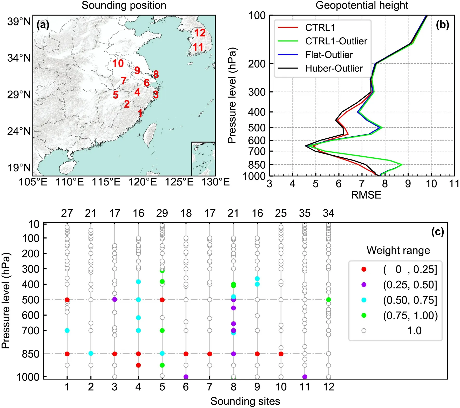
Fig.3.(a) Positions of sounding sites used in the robustness experiments.(b) Vertical profiles of RMSE of geopotential height for CTRL1 (red line),CTRL1-Outlier (green line),Flat-Outlier (blue line),and Huber-Outlier(black line).(c) Vertical distribution of observation weights at the sounding sites in the Huber-Outlier experiment.The top (bottom) of each x-coordinate shows the total number of the assimilated pressures (the site number).

4.Results

4.1.Robustness of variational quality control

Current VarQC methods are based on using contaminated Gaussian distributions to robustly handle outliers.To explore the actual robustness of two VarQC methods,four experiments were designed to assimilate pressure observations by including/excluding outliers as listed in

Table 1

.

Figure 3a

shows the position of the sounding sites used in the idealized experiments,which assimilate the same number of pressure observations with the vertical level up to 10 hPa,as shown in

Fig.3c

.Over the domain in

Fig.3a

,the ERA-Interim reanalysis pressure level data was used to estimate the root-mean-square errors (RMSEs) of the posterior geopotential height fields of the four experiments (

Fig.3b

).Compared to CTRL1,the RMSEs of CTRL1-Outlier are substantially larger at 500 hPa (400−600 hPa) and 850 hPa (700−1000 hPa).These RMSE increases happened since CTRL1-Outlier assimilated the rebuilt outlier observations near these pressure levels (

Table 1

),but CTRL1 assimilated the normal versions of said observations.In other words,replacing some of the normal pressures with outlier pressures and assimilating the “contaminated” dataset without VarQC algorithms caused a degradation of the posterior geopotential height field.

When the outlier pressures are absorbed in Flat-Outlier,the posterior geopotential height field is also degraded with respect to CTRL1.However,Flat-Outlier’s RMSEs are slightly smaller than those of CTRL1-Outlier near 500 hPa.These results indicate that even with Flat-VarQC method,the inclusion of outlier pressures degraded the posterior geopotential height field.In contrast to CTRL1-Outlier and Flat-Outlier,Huber-Outlier showed no increase in the geopotential height RMSEs when the outlier pressures were included.More encouragingly,in the vicinity of 500 hPa,Huber-Outlier’s geopotential height RMSEs are smaller than those of CTRL1.These results indicate that the Huber-VarQC method has strong robustness against outliers.

To explain why the Huber-VarQC method has strong robustness against outliers,the analysis weights of Huber-VarQC were examined.The analysis weights of Flat-VarQC [Eq.(5)] and Huber-VarQC [Eq.(9)] of the assimilated observations in the experiments are determined at each iteration step by its parameters and intermediate innovation by the VarQC 3DVAR system.The weights from the last iteration are analyzed in this study.Following the discussions of

Anderson and Järvinen (1999)

,we identify observations with weights in the range of (0,0.25] as erroneous,observations with weights in the range of (0.25,0.5] as possibly erroneous,observations with weights in the range of (0.5,0.75]as suspicious,and observations with weights in the range of(0.75,1] as valid.The last-step weights of Huber-Outlier show that all the created outlier pressures were subjected to weight reduction (

Fig.3c

).More specifically,the pressure observations of sites 2 and 5 at the 850-hPa level are reduced from 1 to within (0.5,0.75],meaning that they were identified as suspicious observations.The weight of the pressure observation of site 8 at the 850-hPa level fell from 1 to within (0.25,0.5],meaning that the Huber-VarQC method identified the pressure observation as a possible erroneous observation.Similarly,some of the pressure observations at the 500-hPa level also are identified as suspicious (site 4),possibly erroneous (sites 3 and 8),and erroneous (sites 1 and 5).In other words,the negative impacts of assimilating outlier pressures were mitigated by the relatively small observation weights assigned by the Huber-VarQC method.It should be noted that even though both Huber-VarQC and Flat-VarQC adjusted the pressure observation weights,Huber-Outlier substantially outperformed Flat-Outlier.While the Flat-VarQC method’s weight adjustments resulted in a slight RMSE improvement near 500 hPa,relative to CTRL1-Outlier,all of the pressure observations were assigned weights within (0.75,1.0] (not shown).These large weights indicate that outliers are not well identified.The origin of these large weights is likely due to the fact that the Gaussian plus flat distribution does not match the actual observation error distribution as well as the Huber distribution.Moreover,the Huber-VarQC method also reduced observation weights at pressure levels with no outliers(

Fig.3c

).For example,Huber-VarQC recognized the innovation with a pressure equal to 925 hPa at site 4 (red dot) as erroneous.In other words,the VarQC algorithms also assigns a small weight to observations where the quality of the background field is likely poor.Thus,high-quality initial conditions are required when initiating the VarQC assimilation system.Consequentially,because the Flat-VarQC method had difficulties in mitigating the negative impacts of assimilating outlier pressures and dealing with poor quality background fields,Flat-Outlier did not perform as well as Huber-Outlier.

In summary,the idealized experiments show that the Huber-VarQC method has a substantially stronger capability to recognize outliers than the Flat-VarQC method.This suggests that the Huber-VarQC method is more robust at handling outliers than Flat-VarQC.Also,the Flat-Outlier experiment produced a slightly better posterior analysis than the CTRL1-Outlier experiment because the Flat-VarQC method did adjust the observations’ weights.Finally,the experiments indicate that in the absence of VarQC,outliers that pass CQC can degrade the posterior analysis in the current GRAPES m3DVAR system,as opposed to a posterior analysis generated without outliers.

4.2.Observational weight features

The impacts of the Flat-and Huber-VarQC methods were also examined in the context of assimilating real data.

Figure 4a

shows the three-month statistics for surface pressures in a fashion similar to

Fig.1

.As seen in

Fig.4a

,the three distributions (Gaussian,Gaussian plus flat,and Huber distribution) show a similar fit to the right tail of the innovation distribution.Nonetheless,because the left tail of the innovation distribution (green histogram bars in

Fig.4a

) is fatter than the right tail,the innovation distribution is not fitted well by any of these profiles.This is as expected as fitting symmetrical distributions to asymmetric statistics would result in some failure in the fitting.While it is uncertain that the histogram-estimated innovation left-tail probability density is correct,the current DA with a Gaussian OEDM would treat observations from this regime as valid(weights equal to 1).As such,the inclusion of these observations could bring uncertainty to the posterior analysis.Furthermore,the histogram in

Fig.4a

shows a precipitous cut-off at the −4 magnitude of innovations due to the threshold limit assigned in the current background quality check.This confirms that observation errors after CQC are not guaranteed to be Gaussian-distributed.To examine Huber-VarQC’s ability to handle the uncertainties discussed in the previous paragraph,a special test of Huber-VarQC was performed for 0600 UTC 10 August 2015.In view of the robustness of Huber-VarQC,this test was performed with the same configurations explained in

Table 3

except that the background quality check threshold coefficient was relaxed from 4 to 16.As seen in

Fig.4b

,the relaxation resulted in the extension of the green histogram to stronger negative normalized innovation values,indicating that substantially more surface pressure observations were assimilated.More importantly,most of the weights corresponding to observations in the green histograms are less than 0.25 (

Fig.4b

) and are thus identified as erroneous.Therefore,Huber-VarQC can assign weights based on the observational quality to absorb (reject) the usable (harmful) information of outliers.This suggests that when the Huber-VarQC method is used,the threshold limits in BgQC can be relaxed to assimilate more observations.This way,the uncertainty introduced by assimilating observations with strong negative normalized innovations (left tail in

Fig.4a

) can also be relieved significantly.The sensitivity of the posterior analysis to different threshold limits can be studied in the future.Nonetheless,this particular test indicates that the Huber-VarQC method can robustly handle outlier surface pressure observations.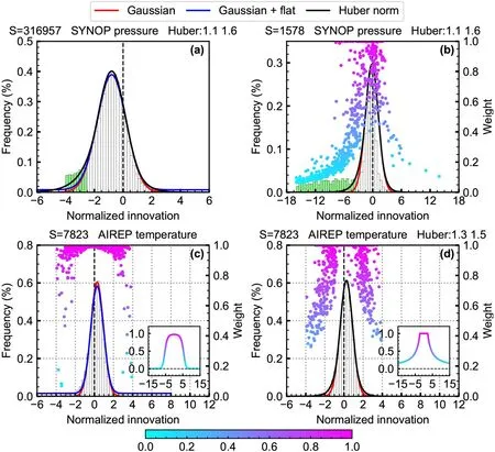

Fig.4.(a) As in Fig.1 but for surface pressure observations from July to September 2013.(b) Statistics of innovations and weights for surface pressure at 0600 UTC 10 August 2015,in a Huber-VarQC test with the background quality check threshold coefficient relaxed from 4 to 16 in the background quality check.(c,d) Statistics of the innovations and weights for aircraft-reported temperature,as assimilated by Flat-VarQC (c) and Huber-VarQC(d).The colored dots represent the magnitude of observation weights in the VarQC methods and correspond to the yaxes to the right.The theoretical weight curves of the two VarQC methods are shown in the bottom-right subplots of panels (c) and (d).The colors of the theoretical weight curves are consistent with the weight colorbar at the bottom of the figure.

To examine the effectiveness of the two VarQC methods in adjusting the observation weights,we assimilated the conventional observations using the two VarQC methods at 0600 UTC on 10 August 2015 but without relaxing the BgQC threshold limits.This time was randomly chosen from the long-period assimilation experiments.

Figures 4c

and

4d

respectively show the last-step observation weights of the aircraft-reported temperature observations produced by Flat-VarQC and Huber-VarQC.As seen in

Figs.4c

and

4d

,the weights assigned by the two VarQC methods have different characteristics.Firstly,in the Gaussian domain,the analysis weights of the Flat-VarQC method are all approximately equal to but less than 1,whereas the Huber-VarQC method’s Gaussian domain analysis weights are exactly equal to 1.When we go beyond the Gaussian domain,the weights of the Flat-VarQC experiment decrease steeply.In contrast,Huber-VarQC’s weights decrease smoothly with increasing innovations.In other words,Flat-VarQC’s weights display an "n" shape [Eq.(5),subgraph in

Fig.4c

],whereas those of Huber-VarQC display a "π" shape [Eq.(9),subgraph in

Fig.4d

].Therefore,these VarQC methods can effectively adjust the analysis weights for real observations.

4.3.Optimization of analysis increment

The analysis increment is the difference between the analysis and the background.Thus,the incremental magnitude can be used as an indicator of how much an observation can correct the background after quality control and data assimilation.This incremental response can also reveal the influence of variational quality controlled observations.The differences in 850-hPa geopotential height increment magnitudes between Flat-VarQC/Huber-VarQC and CTRL2 are shown in

Fig.5

.Note that the increment magnitude characteristics of the geopotential height and temperature fields are similar(not shown).The two VarQC methods have distinctly different impacts on the analysis increment of the geopotential height as compared to CTRL2.The signs of the increment magnitude differences in

Fig.5

are consistent between both VarQC methods in most regions.However,in regions where both VarQC methods have larger increment magnitudes than CTRL2 (red shaded regions in

Figs.5a

and

5b

),Flat-VarQC has noticeably larger increment magnitudes than Huber-VarQC.Furthermore,in regions where both VarQC methods have smaller increment magnitudes than CTRL2 (green shaded regions in

Figs.5a

and

5b

),Huber-VarQC has noticeably smaller increment magnitudes than Flat-VarQC.Taken together,these increment magnitude differences imply that Flat-VarQC generally has larger increment magnitudes than Huber-VarQC.The observational weights generated by Flat-VarQC and Huber-VarQC are also plotted in

Fig.5

.While the two VarQC methods utilize different observational error distributions,the reduction of the observational weight for Flat-VarQC and Huber-VarQC occurs at the same or adjacent stations.The observations in Flat-VarQC,whose weights fall in the range of (0.75,1] and are flagged by grey circles,are in locations similar to those of Huber-VarQC.However,there are differences between the two VarQC methods’weights.Observations with weights under 0.75 are spaced further apart in Flat-VarQC than those of Huber-VarQC.Furthermore,Flat-VarQC’s sub-0.75 weights tend to be smaller than those of Huber-VarQC.From these results,we can infer that Huber-VarQC is more inclusive than Flat-VarQC.Aside from that,

Fig.5a

reveals that the absolute differences between the increment magnitudes of Flat-VarQC and CTRL2 are stronger around observations with reduced weights.This tendency is particularly noticeable around observation sites with severe weight reduction.A similar pattern can be seen with the Huber-VarQC method (

Fig.5b

).In other words,for both VarQC methods,the higher the weight reduction,the greater the change in increment magnitude around the weight-reduction sites.As we will see in the next section,this pattern improved the analyzed geopotential height field relative to CTRL2.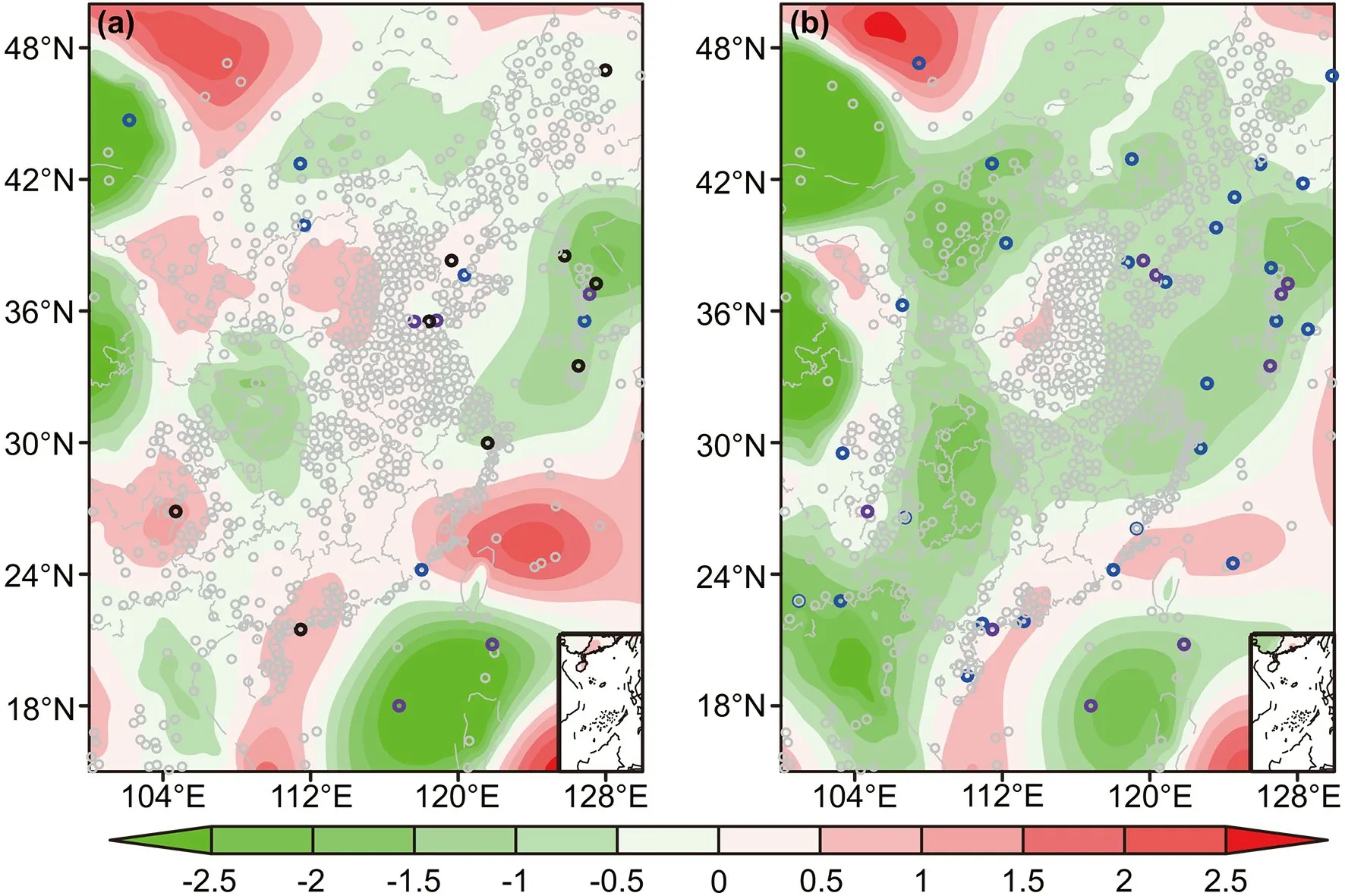

Fig.5.Differences in analysis increment magnitudes for geopotential height (units:gpm) at the 850-hPa level between the Flat-VarQC/Huber-VarQC and the CTRL2 experiments at 0600 UTC 16 August 2015.(a) Flat-VarQC minus CTRL2,(b) Huber-VarQC minus CTRL2.The small circles indicate the VarQC weights of pressure observations at sites from TEMP,SYNOP,and SHIP data.The black circles represent erroneous observations with weights within (0,0.25],the purple circles represent potentially erroneous observations with weights within(0.25,0.5],the blue circles represent suspicious observations with weights within (0.5,0.75],and the grey circles represent valid observations with weights within (0.75,1].

4.4.Improvement of mass field

The improvement of initial conditions is critical to improving model forecasts.

Figure 6

shows the differences between the CTRL2,Flat-VarQC,and Huber-VarQC experiments and ERA-Interim reanalysis for geopotential height at 850 hPa for 0600 UTC 16 August 2015,which is after one DA cycle.We use the ERA-Interim reanalysis as our validating truth.The smaller the difference,the closer the geopotential height is to the ERA-Interim reanalysis.The results from the three experiments are noticeably different from the ERA-Interim reanalysis.These differences are especially large over the middle-west and northern parts shown in

Fig.6

,where the maximum difference is about 20 geopotential meters (gpm).Over other areas,the simulations from the GRAPES model are closer to ERA-Interim with a difference within about 5 geopotential meters.We now compare the experiments against each other.Compared to CTRL2,the differences between the VarQC experiments and ERA-Interim are smaller over most regions(

Figs.6b

and

c

).These regions,which include the regions marked by black ellipses,are also areas in the vicinity of reduced-weight observations.Another point of interest is that the Huber-VarQC method’s posterior analysis is closer to the truth than that of Flat-VarQC.For example,even though the Flat-VarQC method only identified one erroneous observation (black circle) in the ellipse regions of the bottom-left corner of

Fig.6b

,the resulting analysis over the Sichuan province was further from the ERA-Interim than that of CTRL2.In contrast,over the same regions,the Huber-VarQC method identified four observations for which the weights are reduced (one possible erroneous observation and three suspicious observations) and resulted in a deviation from ERA-Interim that is smaller than both CTRL2 and Flat-VarQC.More notably,the Huber-VarQC method reduced the geopotential height deviation from ERA-Interim to about 9 gpm (as opposed to about 13 gpm in other experiments) without treating any of those observations as erroneous.Aside from the region marked by the lower-left black ellipse,the Huber-VarQC results are also closer to ERAInterim in the other regions marked by black ellipses,as compared to the Flat-VarQC results.This suggests that the increment response (

Fig.5

) to the weight-reduction of observations made the geopotential height closer to the ERAInterim reanalysis in the VarQC experiments,particularly for Huber-VarQC.The temperature shows a similar performance (not shown).Similar improvements are also observed for geopotential heights at most other pressure levels(shown in

Figs.7

and

8

).

Figure 7

shows the vertical profiles of geopotential height RMSE for the three experiments at 0600 UTC on 16 August 2015,using the ERA-Interim reanalysis as the benchmark.The RMSEs of geopotential height from the two VarQC experiments are noticeably smaller than those of CTRL2 at most levels,and the Huber-VarQC method has the smallest RMSE.The best performance in Huber-VarQC is consistent with the idealized experiments (

Fig.3b

).This is because the Huber-VarQC method can assimilate outliers more robustly than Flat-VarQC while mitigating non-Gaussian observation errors' negative impacts.Furthermore,the VarQC experiments performed better at the lower-to-middle levels than at the middle-upper levels (200−500 hPa).This improvement is also seen in the long period DA experiments (

Fig.9

).This improvement in the long period DA experiments is probably because the Huber-VarQC method in the GRAPES m3DVAR system used the unchanged transition points at different levels based on the discussion by

Tavolato and Isaksen (2015)

.

Fig.6.Differences of posterior analysis for geopotential height (units:gpm) between (a) CTRL2,(b) Flat-VarQC,(c) Huber-VarQC experiments,and ERA-Interim reanalysis at the 850-hPa level at 0600 UTC 16 August 2015.Circles indicate the weight magnitude at sites,as shown in Fig.5.

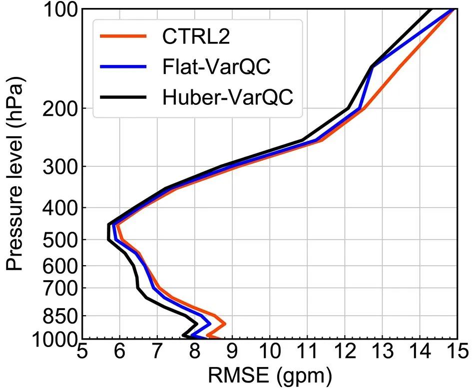
Fig.7.Vertical RMSE profiles of posterior geopotential height for CTRL2 (red line),Flat-VarQC (blue line),and Huber-VarQC (black line) at 0600 UTC 16 August 2015.

To confirm that the Huber-VarQC method generally yields better RMSEs than Flat-VarQC,the two VarQC methods are continuously performed at 0000,0600,1200,and 1800 UTC each day for a total of 31 days over August 2015.The configurations of these VarQC continuous DA experiments and a control continuous DA experiment(CTRL2) are shown in

Table 3

.The ERA-Interim-relative RMSEs of the posterior geopotential height over eastern China (red shaded region shown in

Fig.2

) are shown in

Figs.8

and

9

.The differences of geopotential height RMSE at 850 hPa (

Fig.8a

) and 500 hPa (

Fig.8b

) are calculated with Flat-VarQC and Huber-VarQC minus CTRL2.The more negative the RMSE differences are for a VarQC experiment,the better the performance of said VarQC experiment relative to CTRL2.The 850-hPa geopotential height RMSE differences in

Fig.8a

from the two VarQC experiments are negative at most times,indicating that the VarQC experiments are superior to CTRL2 at 850 hPa.Furthermore,the Huber-VarQC method has smaller 850-hPa geopotential height RMSEs than the Flat-VarQC method most of the time.The RMSE improvement of geopotential height at 500 hPa is not as straightforward as at 850 hPa,but the RMSEs (

Fig.8b

) of Huber-VarQC are still smaller than that of CTRL2 at most times.In general,the RMSEs of Flat-VarQC are better than those of CTRL2.But,Flat-VarQC shows a bad RMSE difference with a value of～2.8 against CRTL2 at 1800 UTC on 26 August.This event is probably because of the convergence issues in the cost function minimization.These findings suggest that the two VarQC methods tested here generally improve the low-level analysis field for geopotential height,especially in the Huber-VarQC experiment,and that the improvements are weaker at middle-upper levels.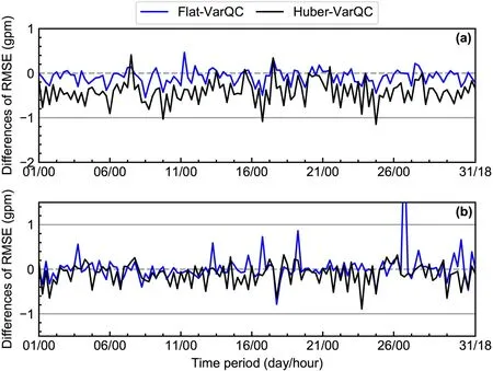

Fig.8.Time evolution of the RMSE differences calculated with Flat-VarQC (blue line) and Huber-VarQC (black line) minus CTRL2 for posterior geopotential height at (a) 850 hPa and (b) 500 hPa,spanning August 2015.

The mean of vertical profile RMSE for geopotential height from the long period experiments over August 2015 is shown in

Fig.9

.Both Flat-VarQC and Huber-VarQC improve the geopotential height at low-middle levels(500−1000 hPa),with the latter VarQC method producing greater improvements.In middle-upper levels,the RMSE of both VarQC methods is similar to the control experiment.The RMSE profiles of temperature also show similar performances,but weaker (not shown).These results indicate that the initial version of VarQC needs to be further improved.For instance,the parameters of the left-and right-transition points in the Huber-VarQC method can vary with height.However,in these experiments,these parameters are fixed.Further study is needed to refine the usage of these parameters.

5.Conclusion and discussion

The VarQC method is a powerful tool for treating outliers that would otherwise amplify uncertainties in variational assimilation or be discarded.Since VarQC is integrated into VarDA’s optimization process,VarQC can iteratively remediate the deficiencies of CQC.In this study,we derived the equations governing a VarQC method that utilizes a Gaussian plus flat CGD,as well as the equations that govern a VarQC method that utilizes a Huber norm CGD.Following that,we implemented these two VarQC methods(Flat-VarQC and Huber-VarQC) in the GRAPES m3DVAR assimilation system based on the actual non-Gaussian innovations.

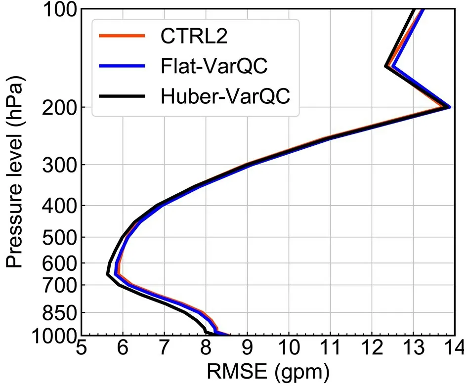
Fig.9.As in Fig.7 but for the mean of RMSE spanning August 2015.

These VarQC methods were then tested in idealized experiments.These experiments show that the Flat-VarQC method lacks robustness against outliers but nonetheless provides a slight improvement over just using CQC to treat outliers.The Huber-VarQC method is more robust than Flat-VarQC because it can accurately identify the outliers and reduce the outliers’ contamination of the posterior analysis.We then demonstrated that the Huber-VarQC method generated a better posterior analysis of the geopotential height compared to the Flat-QC method.

These VarQC methods were then tested with real-data experiments.When the analysis weights in Flat-VarQCs were plotted with respect to innovation,the weights formed an "n" shaped pattern.Likewise,the Huber-VarQC analysis weights formed a "π" shape.These shapes are consistent with the corresponding theoretical curves of Flat-VarQC and Huber-VarQC.Furthermore,the results from the case study indicate that VarQC can have a positive impact on the posterior analysis of the mass field by reducing the weights for uncertain observations (innovations).A subsequent examination of the mass field RMSEs revealed that the Huber-VarQC experiment had noticeably better mass field RMSEs than those of the control and Flat-VarQC experiments.The results of the long period experiment demonstrated that the VarQC experiments performed better at the lower levels than at the middle-upper levels.Finally,the Flat-VarQC experiment does have a better performance than the control experiment,but it does not perform as well as Huber-VarQC.

Our experiments indicate that applying either of the two VarQC methods can improve the analyzed lower level mass field,especially so in the case of Huber-VarQC.However,the two VarQC methods made no noticeable improvements in the mass field at the middle-upper levels.Furthermore,in comparison to the posterior of CTRL2 (not shown),Huber-VarQC shows a favorable performance for specific humidity and wind but Flat-VarQC shows slightly poorer performance compared to CTRL2.Possible reasons for this could be investigated in future work.

Another important avenue of future research concerns applying the VarQC methods to satellite observations.A key challenge with satellite observations is that the innovations often follow non-Gaussian distributions (

Geer and Bauer,2011

;

Harnisch et al.,2016

;

Minamide and Zhang,2017

;

Honda et al.,2018

;

Chan et al.,2020

),which complicates the issue of prescribing a good CGD for VarQC.Aside from that,the radiative transfer observation operators used in assimilating satellite observations are often nonlinear(

Bauer et al.,2011

),especially for infrared observations.This nonlinearity can lead to convergence issues during the cost function minimization.These challenges can be addressed in future work.

Future work can also examine the impacts of using VarQC to assimilate conventional and unconventional observations during complex phenomena (e.g.,precipitation,extreme weather events,and typhoons).Finally,the sensitivity of relaxing threshold limits in Huber-VarQC can be examined in the future,and more studies will be conducted when the variational quality control methods have gained more maturity in the GRAPES m3DVAR system.We will be submitting a companion paper about optimization parameters in VarQC.

The goal of VarQC is to improve forecasts by enhancing our use of outlier observations.With the implementation of our Huber-and Flat-VarQC methods in GRAPES m3DVAR,observations that will otherwise be rejected can contribute to improving forecasts.

:The authors thank Yinghui LU for his helpful advice and grammar correction.Jie HE is supported by the China Scholarship Council.This work is primarily sponsored by the National Key R&D Program of China (Grant No.2018YFC1506702 and Grant No.2017YFC1502000).We acknowledge the High Performance Computing Center of Nanjing University of Information Science &Technology (NUIST) for their support of this work.The datasets in this paper are archived and accessible on the supercomputer of NUIST.