Stochastic frontiers or regression quantiles for estimating the self-thinning surface in higher dimensions?

Dechao Tian·Huiquan Bi·Xingji Jin·Fengri Li

Abstract Stochastic frontier analysis and quantile regression are the two econometric approaches that have been commonly adopted in the determination of the self-thinning boundary line or surface in two and higher dimensions since their introduction to the field some 20 years ago.However,the rational for using one method over the other has,in most cases,not been clearly explained perhaps due to a lack of adequate appreciation of differences between the two approaches for delineating the self-thinning surface.Without an adequate understanding of such differences,the most informative analysis may become a missed opportunity,leading to an inefficient use of data,weak statistical inferences and a failure to gain greater insight into the dynamics of plant populations and forest stands that would otherwise be obtained.Using data from 170 plot measurements in even-aged Larix olgensis (A.Henry) plantations across a wide range of site qualities and with different abundances of woody weeds,i.e.naturally regenerated non-crop species,in northeast China,this study compared the two methods in determining the self-thinning surface across eight sample sizes from 30 to 170 with an even interval of 20 observations and also over a range of quantiles through repeated random sampling and estimation.Across all sample sizes and over the quantile range of 0.90 ≤ τ ≤ 0.99,the normal-half normal stochastic frontier estimation proved to be superior to quantile regression in statistical efficiency.Its parameter estimates had lower degrees of variability and correspondingly narrower confidence intervals.This greater efficiency would naturally be conducive to making statistical inferences.The estimated self-thinning surface using all 170 observations enveloped about 96.5% of the data points,a degree of envelopment equivalent to a regression quantile estimation with a τ of 0.965.The stochastic frontier estimation was also more objective because it did not involve the subjective selection of a particular value of τ for the favoured self-thinning surface from several mutually intersecting surfaces as in quantile regression.However,quantile regression could still provide a valuable complement to stochastic frontier analysis in the estimation of the self-thinning surface as it allows the examination of the impact of variables other than stand density on different quantiles of stand biomass.

Keywords Larix olgensis·Normal-half normal distribution·Site productivity·Woody weeds·Sample size·Quantile selection

Introduction

In plant population and community ecology,self-thinning refers to the progressive decline in stand density (i.e.number of plants per unit area) through competition-induced mortality as individual plants grow larger and collectively accumulate more biomass while competition intensity increases and site resources become limiting for all to survive (Harper 1977;Begon et al.2006).A series of Japanese studies on density effects,intraspecific competition and self-thinning among plants over a decade soon after the Second World War gave rise to the self-thinning rule for even-aged plant populations (Kira et al.1953;Koyama and Kira 1956;Shinozaki and Kira 1956;Yoda et al.1957,1963).The rule delineates a density-dependent upper frontier of mean plant mass or total stand biomass for even-aged pure stands at full site occupancy in a given environment with a power function:

where B represents either mean plant mass or the total stand biomass per unit area,N is stand density,Kis a speciesspecific and environment-specific constant,andβ1is the selfthinning exponent,postulated to be −1.5 for mean plant mass or −0.5 for total stand biomass (Yoda et al.1963;White and Harper 1970;White 1980,1981,1985;Westoby 1984;Whittington 1984).When plotted on a log–log graph,this power function becomes the self-thinning boundary line that regulates the growth trajectories of even-aged plant populations from herbs to trees in the two-dimensional space of log transformedBandN(Gorham 1979;Norberg 1988;Pretzsch 2002).For trees in forest stands managed for timber production in particular,the quadratic mean dimeter (Dq),an easily obtainable stand attribute,is often used instead of average tree mass or stem volume as a measure of average tree size in the determination of size-density relationships for stand density management.In this case,the maximum size-density relationship of Reineke (1933),which defines a species-specific upper limit of stand density for a given quadratic mean diameter on log scales,has proven to be a special case of the self-thinning boundary line (Pretzsch 2002,2009;Pretzsch et al.2012).

For quite some time in much of the earlier literature,it was generally understood that the self-thinning boundary line was species-specific and site-independent as reviewed by Westoby (1984).This presumed invariability with soil fertility or site productivity was largely due to the limitation of the original simplistic graphical analysis of the classic self-thinning experiment by Yoda et al.(1963),where a single boundary line was drawn visually on top of the self-thinning trajectories of horseweed (Erigeron canadensis(L.) Cronquist) populations grown at different levels of soil fertility.A statistically more rigorous analysis of the same experimental data by Bi (2004) some forty years later revealed that the intercept of the self-thinning boundary line increased with soil fertility.This revelation effectively extended the originally presumed species-specific twodimensional boundary line into a three-dimensional selfthinning surface over a gradient of soil fertility.Such a surface was also observed in even-aged forest stands of both coniferous and broadleaf tree species (Bi 2001;Weiskittel et al.2009;Zhang et al.2013).In addition to soil fertility or site productivity,other environmental and climatic variables as well as stand type and history have been found to influence the self-thinning boundary line (Weiskittel et al.2009;Zhang et al.2013;Brunet-Navarro et al.2016;Condés et al.2017;Kweon and Comeau 2017;Andrews et al.2018).Furthermore,attempts have been made to delineate the boundary line for uneven-aged or mixed-species stands(Puettmann et al.1992;Woodall et al.2003,2005;Ducey and Knapp 2010;Long and Shaw 2012;Rivoire and Le Moguedec 2012;Reyes-Hernandez et al.2013;Brunet-Navarro et al.2016;Andrews et al.2018;Bravo-Oviedo et al.2018;Quiñonez-Barraza et al.2018;Salas-Eljatib and Weiskittel 2018;Weiskittel and Kuehne 2019;Kimsey et al.2019;Herberich et al.2020).These developments have further extended the three-dimensional self-thinning surface exemplified by Bi (2001,2004) into higher dimensions:

whereX’s are other independent variables indexed byi=2,…,Iin addition to stand density.

The delineation of the two-dimensional self-thinning boundary line has mostly in the past relied heavily on either visual or more systematic selection of data points that lie close to a perceived or arbitrarily determined upper boundary (Bi and Turvey 1997;Solomon and Zhang 2002;Sun et al.2010;Deng and Li 2014;Brunet-Navarro et al.2016;Ge et al.2017).

Only the selected data are then used to formally delineate the perceived boundary line through traditional methods such as least squares regression or principle component analysis (e.g.,Bi and Turvey 1997;Zhang et al.2005;Marchi 2019).However,no matter how data selection is done,some degree of subjectivity cannot be avoided,resulting in a certain lack of objectivity in the estimated self-thinning boundary line.To overcome this problem,two econometric methods,namely stochastic frontier analysis (SFA) and quantile regression (QR),were introduced to the estimation of the self-thinning boundary line by Bi et al.(2000),Bi (2001,2004),Cade and Guo (2000) and Zhang et al.(2005).These two methods have since become the most commonly used techniques for estimating the self-thinning boundary line or surface in two and higher dimensions.Stochastic frontier analysis has been performed in some studies (e.g.,Montigny and Nigh 2007;Weiskittel et al.2009;Charru et al.2012;Reyes-Hernandez et al.2013;Kweon and Comeau 2017;Quiñonez-Barraza et al.2018;Kimsey et al.2019),while quantile regression has been carried out in others(e.g.,Vospernik and Sterba 2015;Xue et al.2015;Riofrío et al.2016;Condés et al.2017;Andrews et al.2018).In far fewer studies,both methods have been used (Sun et al.2010;Zhang et al.2013;Salas-Eljatib and Weiskittel 2018).

Among these studies,the number of independent variables other than stand density that were incorporated into the model specification generally in the form of Eq.2 has varied between one and four (e.g.,Weiskittel et al.2009;Reyes-Hernandez et al.2013;Zhang et al.2013;Kweon and Comeau 2017).Concomitantly,the number of data points ranged from tens to hundreds and thousands (e.g.,Comeau et al.2010;Sun et al.2010;Zhang et al.2013;Condés et al.2017;Kweon and Comeau 2017),and even to more than ten thousand in the extreme case (Vospernik and Sterba 2015).However,the rational for using stochastic frontier analysis or quantile regression has in most cases not been clearly explained and there appears to be a general lack of adequate appreciation of the differences between the two methods as statistical estimators for delineating the self-thinning surface.Without a thorough understanding of such differences,the best and most informative method for analysing the valuable empirical data at hand may become a missed opportunity,leading to an inefficient use of data,a failure to gain a greater insight into stand dynamics that would otherwise be obtained from the analysis,and more practically,leading to a suboptimal stand density management scheme for evenaged forest plantations.Even more seriously,the validity of results may be called into question if statistical inferences are not made on a valid or reliable basis.

The two methods were brief ly compared by Zhang et al.(2005) in a short research note for estimating the self-thinning boundary line using 262 data points from even-aged pure stands of eastern white pine (Pinus strobusL.) as an example.Following this initial work,two brief comparisons of the methods were reported by Sun et al.(2010) and Zhang et al.(2013).The former used 160 observations from 10 experimental plots that were repeatedly measured in a spacing trial of Chinese fir (Cunninghamia lanceolata(Lamb) Hook.),and the later analysed data of ponderosa pine (Pinus ponderosaLawson &C.Lawson) from 109 long-term research plots and 59 temporary inventory plots across California.In addition,the study by Socha and Zasada (2014) on the allometric relationships between density and tree dimensions in birch stands on postagricultural lands in Poland also contained some comparative results.A further and more considered comparison of these two methods was made in a recent study by Salas-Eljatib and Weiskittel (2018),particularly for determining the maximum stand density,i.e.the maximum number of trees at a given reference average diameter,using 178 observations from 130 plots in mixed Nothofagus forests.

All these comparisons have been made in a two-dimensional space,except for Zhang et al.(2013) which included site index in the analysis and were limited to the comparative positions of the estimated self-thinning boundary line.The methodological attributes and statistical properties of the two approaches that researchers need to carefully consider before choosing one or the other for their particular research objectives and for the nature and size of data at hand remain to be further evaluated,particularly when the analysis goes beyond two dimensions.This paper aimed to further evaluate and highlight the pros and cons of these two methods particularly for estimating the self-thinning surface in higher dimensions through a more detailed comparison across a range of data sizes,(i.e.number of data points),to help researchers make the best choice for their analyses.In doing so,the two econometric methods were brief ly reviewed first to provide the minimum but most essential details on their statistical properties as parametric boundary estimators.They were then compared in the estimation of the self-thinning surface in higher dimensions using cross-sectional data from even-agedL.olgensisplantations across a range of sample sizes through repeated random sampling with replacement and model estimation.Finally,some practical guidance for choosing the best method is provided for researchers to address their particular research questions.

Materials and methods

Stochastic frontier analysis and quantile regression

Stochastic frontier analysis originated from the economic concept of a production function which relates an upper boundary of maximum attainable output to any given quantities of a set of inputs in a production process (see Farrell 1957;Forsund et al.1980;Schmidt 1985).This econometric approach was first proposed some 40 years ago by Aigner et al.(1977),Battese and Corra (1977) and Meeusen and van den Broeck(1977).Over the past four decades,it has been intensively studied and applied to the estimation and measurements of productivity and technical efficiency in economics and a very wide range of other fields (see Kumbhakar and Lovell 2000;Fried et al.2008;Kumbhakar et al.2018 for major reviews).The model specification commonly used for a stochastic frontier function takes the form of what is known in economics as the Cobb–Douglas production function with a composed error structure:

where Y is the dependent variable which is called output in econometrics,X’s are inputs,i.e.,independent variables,Aandβ’s are parameters,evande−uare two error components.Taking logarithms,the model becomes

wherey=lnY,α=lnA,lndenotes natural logarithm,Xis a vector of log-transformed independent variables,and β is a vector of parameters.The composed error term,ε=v−u,is a compound random variable with two components and each is assumed to be independently and identically distributed across observations.The first error component ν is assumed to be normal with zero mean and constant varianceσ2vand is intended to capture the effects of random factors external to producers on the frontier.The second random variable u is non-negative and is specified to capture the effects of technical efficiency of producers.Becauseu≥0,it was assigned a half-normal distribution and an exponential distribution in the three seminal papers published in 1977,effectively giving the stochastic frontier function a normal-half normal and a normal-exponential specification.By allowinguto follow a truncated normal distributionN+(μ,) obtained by truncating at zero of the normal distribution with meanμand varianceStevenson (1980) generalised the normalhalf normal model into a normal-truncated normal specification for a more flexible representation of the patterns of technical efficiencyuin the data.The flexibility is realised because the mode ofuin the truncated normal distribution is no longer arbitrarily set at zero,but is allowed to be estimated together with other parameters in the stochastic frontier model.Unlike the half-normal and exponential densities which always have a mode at 0,the truncated-normal density has a mode at 0 only whenμ≤0,but a mode atμotherwise.

Becauseu≥0 by specification,the composed error term,ε=v−u,is asymmetric and its expectation,E(ε)=−E(u)≤0,asvanduare distributed independently of each other.As shown in Kumbhakar and Lovell(2000):

for the normal-half normal model,and

for the normal-exponential model.For the normal-truncated normal model:

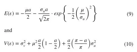
where the pre-truncation mean parameterμbecomes the mode of the truncated normal distribution,is the pretruncation variance of normal distributionN(and Φ(⋅) is the standard normal cumulative distribution function.

Similar to the half normal distribution,the exponential distribution is also a special case of the truncated normal distribution,and as such the three most commonly used distributions foruare all captured by the truncated normal distribution (Meesters 2014).Although other alternative distributions have been proposed foruin econometrics research over the past four decades,stochastic frontier models based on the three distributions,particularly the normal-half normal model,have remained the choice of applied researchers in the vast majority of empirical work (Kumbhakar and Lovell 2000;Parmeter and Kumbhakar 2014;Kumbhakar et al.2018).The model parameters can be estimated by the maximum likelihood method,of which comprehensive descriptions can be found in Aigner et al.(1977),Stevenson(1980),Greene (1997),Kumbhakar and Lovell (2000) and Kumbhakar et al.(2018).

Another econometric approach that lends itself to boundary estimation is quantile regression introduced by Koenker and Basset (1978) at almost the same time when stochastic frontier analysis was first proposed.As reviewed by Kumbhakar et al.(2018) and shown by references therein,it has recently been embraced for the estimation of production frontiers and measurements of efficiency.Quantile regression extends the least squares regression framework,traditionally focused on the conditional mean function onto noncentral parts of the conditional distribution so that theσth quantileQσ(X) of the conditional probability distribution of a response variable Y given X,a vector of predictor variables,can be estimated for any chosen value of 0＜σ ＜1 (Koenker and Hallock 2001;Koenker 2005,2017).The estimator ofQσ(X) proposed by Koenker and Basset (1978) minimises the following asymmetric loss function:

which gives positive and negative residuals the weight ofσand 1 −σ,respectively.The minimization is achieved through linear programming as detailed by Koenker (2005)and Davino et al.(2013),and as such avoids assumptions of error distributions that are required by stochastic frontier models.

The quantile regression estimator is consistent and asymptotically normally distributed under some regularity conditions (Koenker and Basset 1978).Under the assumption of independent and identically distributed (i.i.d.) errors,its asymptotic variance–covariance matrix can be obtained analytically through the estimation of the so-called sparsity function by differentiating a theoretical quantile function or by using a difference quotient of empirical quantiles.In the case of non i.i.d.errors,the derivation is more complicated as it uses a local estimate of the sparsity function to compute a Huber sandwich estimate (Koenker 2005;Hao and Naiman 2007).To avoid making the i.i.d.assumption,which is often not the case in quantile regression applications,and still obtain robust results,resampling methods such as bootstrapping are commonly implemented in quantile regression applications (Kocherginsky et al.2005;Koenker 2005;Hao and Naiman 2007;Tarr 2012).As the estimator uses a wellknown M-function,the absolute value function,it is robust or more resistant than the traditional least squares estimator to the influence of outliers,particularly for inner quantiles.However,the variance of quantile regression estimator is U-shaped withτchanging from zero to one.The implication of such a pattern of estimator variance for extreme quantiles close to the data boundary is that the estimated frontiers or boundary lines can be quite variable even with a very small change in τ,particularly when data are sparse around the edges,and may even cross over each other,posing difficulties for statistical inferences and interpretation of results.

Data

The data set for this study came from 146 temporary square or rectangular plots established between 1991 and 2016 in even-aged larch (L.olgensis) plantations under the management of four forestry agencies across two provinces in northeast China:Mengjiagang (MJG) Forest Farm,Linkou(LK) and Dongjingcheng (DJC) Forestry Bureaux in Heilongjiang Province,and Songjianghe (SJH) Forestry Bureau in Jilin Province.These plots covered much of the natural distribution of the species in northeast China (see Peng et al.2018),and a wide range of site quality and climatic conditions (Table 1).The exact initial planting densities of the individual plots are unknown but they were most likely to be 3300,4400 and 6600 ind.ha−1,the most common planting densities for larch plantations in northeast China (Yu 2008).For planting densities at such high levels,the plot size of 0.04‒0.09 ha would contain enough trees for summarizing key stand attributes and describing stand structure and dynamics,although larger plots would be preferable (see García 1998;García and Batho 2005;Wagner et al.2010;Zhou et al.2019).Some plots were in plantations that had been thinned many years prior to measurement as judged by stumps remaining on the forest floor,but their silvicultural histories were not recorded.Although in even-aged plantations,there were only 38 plots where larch was theonly species.In the remaining plots,larch was the dominant species in both number and size,as naturally regenerated non-crop trees had emerged and mostly grown under the dominant larch,possibly reflecting the differences in previous land use and in site preparations across the plantations.Such non-crop trees in commercial plantations are usually regarded and termed as woody weeds in forest research and management (e.g.,Bi and Turvey 1994;Rose et al.2006).The woody weeds included Korean pine (Pinus koraiensisSiebold &Zucc.) and three broadleaf species:Betula platyphyllaSukaczew,Quercus mongolicaFisch.ex Ledeb.andPopulus davidianaDode.As mostly small trees,they represented less than 30% of the total number of trees and less than 30% of the total stand basal area in most plots (Table 1).

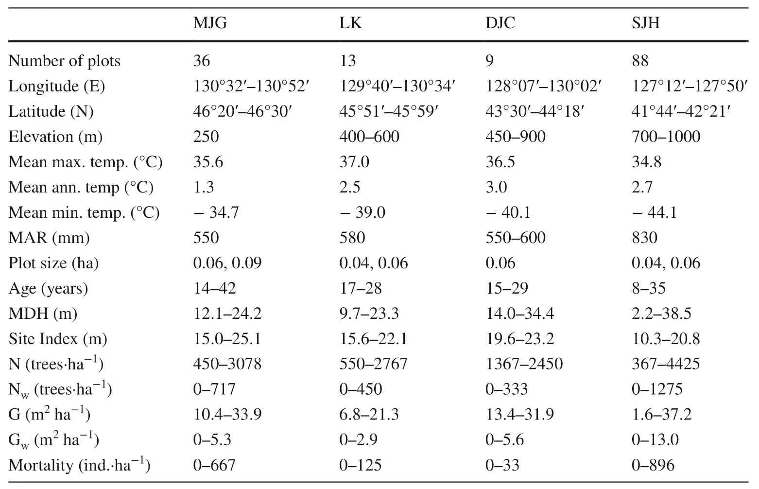
Table 1 Number of plots,geographical locations,plot size,age ranges,key stand attributes and climatic conditions across four forest management areas:Mengjiagang (MJG),Linkou(LK),Dongjingcheng (DJC) and Songjianghe (SJH)

Except for 24 plots on the MJG Forest Farm which were measured twice,all plots had a single measurement for a total of 170 plot measurements from the 146 plots.For the purpose of this paper,the potential correlation between the consecutive measurements of the 24 plots were not taken into consideration.The 170 plot measurements were effectively treated as cross sectional data.Diameter overbark at breast height of 1.3 m above ground (DBH) and total height of all live trees were measured,regardless of species and size.For standing dead trees,only DBH was recorded.At the time of plot measurement,stand age ranged from 8 to 42 years,which was close to the rotation age of 45‒50 years for larch plantations in this region,and stand density varied between 367 and 4425 trees/ha (Table 1).Stand mean dominant height,calculated as the mean height of the 100 tallest trees per hectare,ranged from 2.2 to 38.5 m among the plots.With the calculated stand height and age,site index at the base age of 30 years was derived for each plot using the site index equation developed by Peng et al.(2018) for the same larch species in northeast China.

The aboveground biomass of individual larch trees was calculated from their DBH and total tree height using two sets of biomass equations.The first set was a system of additive biomass equations developed by Dong et al.(2016) based on data from 90 trees with DBH ranging from 7.6 to 35.7 cm from 17 plots in larch plantations in Heilongjiang province.The second set was developed by Zheng and Li (2013) using data from 150 trees with DBH between 1.6 and 44.1 cm from both plantations and natural forests over a much broader area in northeast China as part of the Eighth National Forest Inventory.As the biomass equations of Dong et al.(2016) were not intended for very small trees,the equations of Zheng and Li (2013)were used to calculate the aboveground biomass of trees with DBH ＜ 5 cm.For larger trees,both sets of equations were used and the two biomass estimates were averaged for each tree and taken as its final biomass estimate.This simple form of model averaging was used to reduce possible prediction bias from arbitrarily choosing any one set of equations.The biomass estimates of individual larch trees were summed up for each plot and converted to total aboveground stand biomass on a pro rata basis.Standing dead trees were not included in the biomass calculation.

Deterministic model specification and estimation

The deterministic model specification extended that of Bi(2001) for estimating the self-thinning surface by incorporating stand density and basal area of non-larch species in the equation:

whereBrepresents stand biomass of larch trees in kg ha−1,Kis a constant,N stands for the stand density of larch in trees/ha,β1is the self-thinning exponent,S is a relative measure of site productivity and takes any value between 0 and 1 because it was calculated as a ratio between site index and the maximum site index of 26 m for larch plantations in northeast China,W is a relative measure of the abundance of woody weeds in the larch stands,β2andβ3are parameters.The formulation of W was based on a still-to-be published study by the second author on self-thinning in relatively even-aged eucalypt regrowth forests in Australia.It took both the density and basal area of woody weeds in the larch stands into account:

whereNwis the density of woody weeds in trees/ha,GandGWindicate,respectively,the basal area of larch and that of woody weeds in m2ha−1.

This formulation ofWwas used following an exploratory analysis with the aim to overcome the collinearity that arose from the correlation betweenNwandGWif the two variables were included separately in the model specification.The ill effects of collinearity on parameter estimation and interpretation in linear regression was well recognised and described by Belsley (1991).In pure larch stands,W=0 ;when woody weeds are present,0＜W ＜1 .WhenW=0 in Eq.(6),woody weeds have no influence whatsoever on the self-thinning surface;whenW ＞0,however,they are expected to have a negative impact on the self-thinning surface because of their competition with larch for site resources.Varying between 0 and 0.82,the calculated W had a positively skewed distribution with a median of 0.12,a mean of 0.18,a third quartile of 0.30 and a 90th percentile of 0.46 (Fig.1).

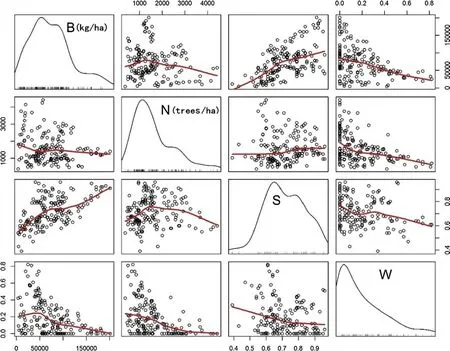
Fig.1 Scatter plot matrix of stand biomass (B),stand density (N),relative site productivity index (S) and abundance of woody weeds (W) for 170 even-aged larch stands;frequency distributions of the four variables are displayed as kernel density plots in the diagonal graphic cells

Estimating the self-thinning surface as stochastic frontiers

To estimate the self-thinning surface as stochastic frontiers in the four-dimensional space,Eq.(12) was linearized by taking the natural logarithm of both sides and the linearized equation was then given a composed error termε=v−u:

wherek=lnK,and the other variables are as previously defined.While the first error component,v,was assumed to followN(0,) as reviewed previously,the second error component,u,was considered to follow either a half normal,or an exponential or a truncated normal distribution.The combination of distributional assumptions of the two error components led to three stochastic frontier models,namely,normal-half normal (NH),normal-exponential (NE) and normal-truncated normal (NT).The three models were estimated through the maximum likelihood estimation using the Quasi–Newton method in the QLIM procedure of SAS/ETS(SAS Institute Inc.2014).Convergence was easily reached for the first two simpler models with no more than 20 iterations.Their parameter estimates and asymptotic standard errors were compared,together with their model fit summaries.However,convergence was not attained for the more complex NT model even after 200 iterations.To overcome the problem of non-convergence and obtain valid parameter estimates,the model was repeatedly estimated 2000 times,each time using 170 observations randomly sampled with replacement from the data set.Using the parameter estimates from the converged cases out of the 2000 rounds of estimation,the mean and standard error were calculated for all model parameters and taken as their parameter estimates and standard errors.Finally,values of,i.e.,estimated residuals of the composed error termεin Eq.(14),were obtained for the three stochastic frontier models.Their residual frequency distributions were then plotted and examined with the aid of simple descriptive statistics including the mean,variance,skewness and kurtosis.

Estimating the self-thinning surface as regression quantiles

Like the stochastic frontier models,Eq.12 was similarly linearized for estimating the self-thinning surface as regression quantiles:

whereBσ,kσ,β1σ,β2σ,andβ3σare previously defined variable and parameters corresponding to the chosen quantileσ.But unlike the composed error term in the stochastic frontier models,εσhere represents theσth quantile of the error term,which is set to zero as required by the model specification of quantile regression (Hao and Naiman 2007).As such,σalso indicates the proportion of nonpositive residuals,or in other words,the proportion of data points on or under the self-thinning surface as defined by theσthconditional quantile oflnBσfor any given values ofN,SandWin Eq.(15).As there were 170 data points available for estimating the self-thinning surface in this study,10 values ofσfrom 0.90 and 0.99 with an even increment of 0.01 were used in the QUANTREG procedure of SAS/STAT (SAS Institute Inc.2013).For the parameter estimates associated with each value ofσ,their approximate standard errors and 95% confidence limits were computed using the resampling method through 2000 repetitions.

Comparative performances of the two methods across sample sizes

The estimations described above used all 170 observations and so the performances of stochastic frontiers and regression quantiles could only be compared on the basis of one sample size.However,as evident from the literature reviewed previously,the sample size,i.e.,the number of observations or data points,used in the estimation of the self-thinning frontiers varied from as small as 30 observations to as large as thousands,even tens of thousands of plot measurements in the extreme case (e.g.Bi 2004;Condés et al.2017;Kimsey et al.2019).As statistical estimators,the two methods would naturally differ in statistical efficiency and so their comparative performances can be expected to change with sample size from small to large.For a more complete and informative comparison of the two methods,the estimations described above were carried out over a range of sample sizes through repeated random sampling with replacement from the 170 observations.In doing so,the sample size varied from 30 to 170 with an even interval of 20 observations and for each sample size the sampling was repeated 2000 times.Each time,the self-thinning surface was estimated as stochastic frontiers as well as quantile regression.As there were little differences in the estimated self-thinning surface among the three stochastic frontier models,only the normal-half normal model was used in the comparison for the sake of parsimony.Considering the range of sample size,20 values ofσfrom 0.80 to 0.99 with an increment of 0.01 were used in the quantile regression for estimating the self-thinning surface.For each sample size,the distribution of the 2000 estimates of each parameter and its descriptive statistics were obtained for the stochastic frontier model and quantile regression over the 20 selected quantiles.These descriptive statistics included the mean,variance,coefficient of variation,skewness and kurtosis calculated as the excess kurtosis,which is three less than the standardized fourth central moment.They were compared between the stochastic frontier model and quantile regression across the range of sample sizes to evaluate the comparative performances of the two methods.

Results

The self-thinning surface estimated as stochastic frontiers

There were little differences in the estimated self-thinning interceptκand slopeβ1in Eq.14 among the three stochastic frontier models with different distributional specifications for the composed error termε(Table 2).The estimated value ofκwas 15.90 for the normal-half normal (NH) model,15.72 for the normal-exponential (NE) model and 15.95 forthe normal-truncated normal (NT) model.The estimated value ofβ1was −0.48 for the NH model,−0.47 for the NE model and −0.50 for the NT model.All three estimates ofβ1were significantly different from zero but not significantly different from −0.50,the hypothesized self-thinning slope atα=0.05 .The estimated values ofβ2andβ3,the two parameters associated with the relative site productivity S and the abundance of woody weeds W,were,respectively,1.54 and −1.52 for the NH model,1.29 and −1.73 for NE model,1.32 and −1.69 for the NT model.The differences in the three estimates of the same parameter were not significant atα=0.05 .The standard errors of parameter estimates were comparable among the two simpler models,but they were noticeably larger for the NT model (Table 2).When the three estimated self-thinning surfaces were sliced at particular values ofSandWand the resulting self-thinning frontiers plotted together,they were hardly visually distinguishable(Fig.2).

Fig.2 Examples of self-thinning frontiers obtained by slicing the estimated self-thinning surfaces at 3 × 3 values of S and W,respectively,representing low,medium and high site quality and 0,medium and high abundance of woody weeds in even-aged larch stands.Solid red lines represent the stochastic self-thinning frontiers resulting from the NH,NE and NT models;broken blue lines from bottom up are those estimated through quantile regression at σ=0.90,0.95 and 0.99.Numbers on lower right-hand corners are number of data points in the subspace delineated by S being ≤ the value in top stripe of each column and by W being ≥ the value in the right stripe of each row.Solid dots represent pure larch stands with W=0 while open circles stands with woody weeds

Table 2 Parameter estimates and standard errors for the self-thinning surfaces estimated through the three stochastic frontier models with normal-half normal (NH),normal-exponential (NE) and normal-truncated normal (NT) specifications for the composed error term ε as in Eq.14

The estimated value ofσvwas smaller for the NH model than for the NE one (Table 2).Consistent with the stochastic frontier specifications,the distribution ofwas negatively skewed and leptokurtic for all three models (Fig.3).The NH model had only six positive residuals (i.e.,＞0 observations above the estimated self-thinning surface) and a meanof −0.67,while the NE model had 18 such residuals and a meanof −0.56.With 12 positive residuals and a meanof −0.59,the NT model was in the middle of the two simper models.The distribution offor the NH model had a smaller variance and was also slightly less skewed and less leptokurtic than the other two stochastic frontier models for which the variance,skewness and kurtosis ofwere almost the same.

Fig.3 Frequency distributions of residuals of the normal-half normal (NH),normal exponential (NE),and normal-truncated normal (NT) stochastic frontier models (top row) and residuals from the quantile regression at the σ th quantile as indicated by the value in the stripe on top of each panel in the bottom row of the multi-panel display.The number on right of the red vertical line in each panel indicates the number of residuals greater than zero

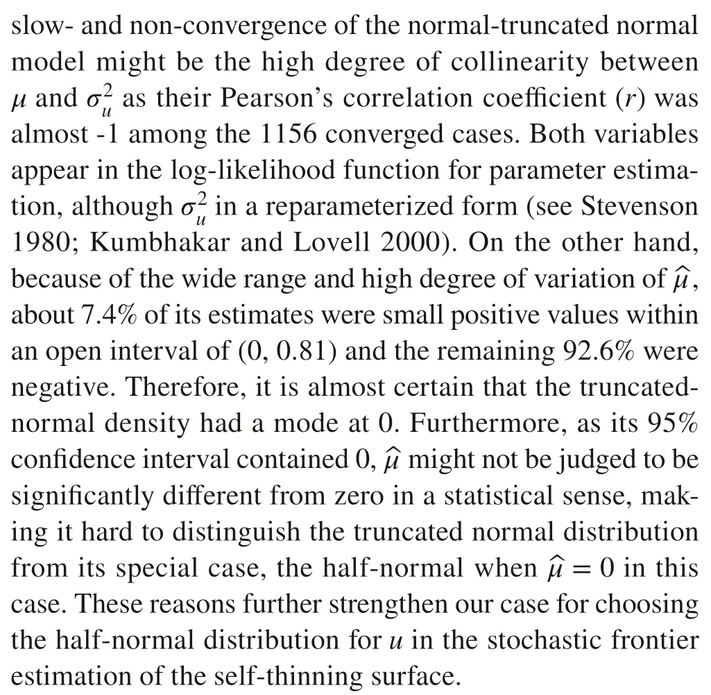
During parameter estimation,convergence was easily reached for the two simpler NH and NE models,but the convergence rate of the NT model was less than 58%,with only 1156 cases attaining convergence out of the 2000 repeated estimations.Among these converged cases,about 7.4% of the estimated mean of the pre-truncation normal distributionwere positive,but only within a narrow open interval of (0,0.81).For the remaining cases,was either a negative or an unreasonably large negative number.The lower 25% values oflay below −12 and even dropped to a 6-digit negative number in the extreme case.The estimates of the pre-truncation standard deviationwere correspondingly large or extremely large,ranging from a single digit to a three-digit number.Pearson’s correlation coefficient betweenwas almost −1,indicating a close negative linear relationship.Among the unconverged cases,the values ofreached when optimization was terminated after a large number of iterations were even larger negative and positive numbers than those in the lower 25% of the estimates of the converged cases as described above.

The self-thinning surface estimated as regression quantiles

Parameter estimates for the self-thinning surface obtained through quantile regression changed systematically asσincreased from 0.80 to 0.99 (Table 3).Among the 20 values ofσ,the parameter estimates and their standard errors wereclosest to the stochastic frontier estimates whenσ=0.80 .Asσincreased from 0.81 to 0.91,the estimated self-thinning interceptkσin Eq.(9) varied within a narrow range between 16.11 and 16.36,while the estimated self-thinning slopeβ1σalso varied narrowly between −0.54 and −0.58.At the same time,the estimates ofβ2σgenerally decreased from values greater than 1.20 to less than 0.90,while the estimates ofβ3σvaried between −1.82 and −2.01.Asσfurther increased beyond 0.91 to 0.99,the parameter estimates for the self-thinning surface exhibited much larger variations.The estimated value ofkσvaried mostly between 15.00 and 16.00 until it dropped down to 13.28 whenσreached 0.99.Correspondingly,the estimated value ofβ1σvaried between −0.36 and −0.51 before it became a much flatter slope of −0.13 whenσ=0.99.The estimated value ofβ2σvaried mostly between 0.57 and 0.94 before reaching a much greater value of 1.11 whenσ=0.99,while that ofβ3σvaried within the range of −2.17 to −1.48 before a large increase to −0.89 at the most extreme quantile.Over the more extreme quantiles,a slight change inσ,even as small as 0.01,could lead to relatively large changes in parameter estimates.As expected,the standard errors of parameter estimates became increasingly larger asσincreased beyond 0.90 to 0.99 (Table 3).Because of the large standard errors,the estimated self-thinning slopeβ1σwas not significantly different from zero atα=0.05 whenσranged from 0.95 and 0.99,and alsoβ2σ,the parameter associated the relative measure of site productivity S.Further detailed numerical and graphical examinations of the self-thinning surfaces estimated at different values ofσrevealed that they intersected each other within the empirical data space delineated in Fig.1,particularly for high and extreme quantiles withσ≥0.90.

Table 3 Parameter estimates and standard errors for the selfthinning surfaces estimated as the σ th regression quantile

Comparative performances of the two methods across sample sizes

Discussion

Since their introduction to the estimation of the self-thinning boundary line some 20 years ago by Bi et al.(2000),Bi (2001,2004),Cade and Guo (2000) and Zhang et al.(2005),stochastic frontier analysis and quantile regression have become the two most commonly adopted econometric approaches by ecologists and forest biometricians in the determination of the self-thinning frontier or surface in two and higher dimensions.The two approaches were both motivated in their early development by the desire to determine an unobservable upper boundary of maximum attainable output for a given vector of inputs in a production processand subsequently to evaluate and benchmark the efficiencies of individual production units against the production frontier (Kumbhakar and Lovell 2000;Parmeter and Kumbhakar 2014;He 2017;Kumbhakar et al.2018).While stochastic frontier analysis has so far been applied predominantly in economics and related fields (Kumbhakar et al.2018),quantile regression,as a natural extension of the traditional least squares regression,has enjoyed a much wider audience and has rapidly become a more general method in applied statistics (Koenker 2005,2017;Hao and Naiman 2007;Davino et al.2013).Although both approaches can serve the same purpose of boundary delineation in applied statistics far beyond econometrics (e.g.,Brandt 2016;Rosenberg et al.2017),the statistical thinking and reasoning behind them are quite different.An adequate appreciation of the differences between the two approaches would be essential for researchers to select the best method to estimate the selfthinning surface,particularly in high dimensions,for their data at hand and to gain a greater insight into how variables other than stand density would impact upon the self-thinning surface.

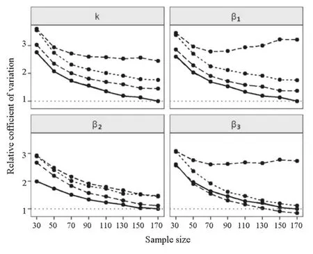
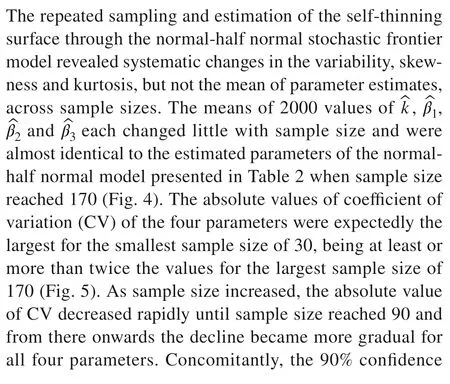
Fig.5 Relative coefficient of variation (RCV) of parameter estimates in relation to sample size for each of the four parameters of the self-thinning surface estimated through the NH stochastic frontier model (solid lines) and by quantile regression with σ=0.90,0.95,0.99 (three broken lines from bottom up in each panel).For each parameter,sample size and estimation method,RCV was the ratio of the coefficient of variation (CV)of 2000 estimates over the CV of parameter estimates obtained through the NH stochastic frontier model using the largest sample size of 170

The three stochastic frontier models,each with a different distributional specification foru,the non-negative one-sided error component in the composed error term of Eq.(14),resulted in little and practically immaterial differences in the estimated self-thinning surface (Fig.2).In this case,a natural question would arise:do distributional assumptions matter in the estimation of self-thinning surface? Despite the vast number of stochastic frontier analysis undertaken in theoretical as well as applied research with empirical data,surprisingly few studies have been devoted to discerning the impact that alternative shapes of the distribution ofucan have on the frontier and efficiency estimation and few attempts have been made to explicitly address specification testing in stochastic frontier models (Guo et al.2018;Kumbhakar et al.2018).Under the assumption of a normally distributedvin the composed error term,Wang et al.(2011) proposed the Pearsonχ2and Komolgorov-Smirnov type statistics to test the goodness of fit of the specific distributional assumption onuthrough simulating the quantiles of the composed error distribution.However,the power of these tests against plausible alternative distributions is somewhat low,making it hard to distinguish the sum of a normal and an exponential from the sum of a normal and a half-normal distribution,unless the variance of the normal component is very small or the sample size is very large(Wang et al.2011).Furthermore,a rejection from the test does not necessarily imply that the distributional assumption onuis incorrect as it could be that the normality distributional assumption onvor the parametric form of the stochastic frontier model is mis-specified (Kumbhakar et al.2018).An alternative test of the distributional assumptions on bothvanduwas proposed by Chen and Wang (2012)through a centred residuals-based method of moments estimator for stochastic frontier models.Unlike the commonly used maximum likelihood estimator for stochastic frontier models,this moment estimator has yet to be implemented in general purpose statistical software.

Philosophically,it does not matter that the stochastic frontier models cannot be distinguished statistically if they give more or less the same results as it only becomes a problem when the models give substantively different results (Wang et al.2011).The choice of a distribution foruout of an ever-increasing number of theoretical candidates such as half normal,exponential,truncated normal,gamma,Pearson,uniform,Beta,Weibull,doubly truncated normal,and even a mixture distribution,as reviewed by Kumbhakar and Lovell (2000),Kumbhakar et al.(2018) and Horrace and Parmeter (2018),is often practically driven through available statistical software to implement the method rather than an underlying theoretical link between a model of productive inefficiency in econometrics and the exact shape of the corresponding distribution.Although conceptually pleasing,some alternative or more complex frontier models may lead to difficult estimation problems as found by Ritter and Simar(1997) with the normal-gamma model and also shown by the difficulty of the NT model in attaining convergence in our case.Possibly as a consequence,the half-normal assumption for the one-sided inefficiency term is almost without question the most common distribution foruin practical applications (Kumbhakar et al.2018).In the case of this study,the estimated variance of the normally distributed error componentfor the NH model was about 60% of that for the NE model based on the estimates ofσvfor the two models (Table 2).Correspondingly there were only six positive residuals for the former against 18 such residuals for the latter.Therefore,the relatively simple half-normal distribution became the obvious choice foruout of the three distributions for estimating the self-thinning surface.

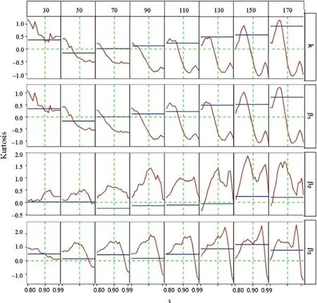
Fig.7 Multi-panel display of the kurtosis of the 2000 estimates for each of the four parameters of the self-thinning surface estimated through the normal-half normal stochastic frontier model (blue lines)and through quantile regression over 20 evenly spaced σ values from 0.80 to 0.99 (red curves) across the eight sample sizes as denoted in the top stripe of each column

Unlike the maximum likelihood-based estimation of parameters in stochastic frontier analysis,quantile regression does not require any distributional assumption to be made for the quantile-specific error termεσas in Eq.(15)because its parameter estimates are obtained by minimising the asymmetric loss function as shown in Eq.(11) through linear programming.However,as shown in Figs.4,6 and 7,the parameter estimates,their variance,skewness and kurtosis were all quantile-dependent and these distributional characteristics also changed with sample size.Consequently,which value ofσto choose for the estimation of the selfthinning surface becomes a question that has to be addressed with sound statistical as well as biological reasoning for the size and nature of the empirical data under analysis.The value ofσchosen for estimating the self-thinning frontier,mostly in the two-dimensional space of stand biomass or tree size versus stand density,has ranged largely from 0.90 to 0.99 in the literature,with 0.95 ≤σ≤0.99 being the most common choices (Sun et al.2010;Zhang et al.2013;Vospernik and Sterba 2015;Xue et al.2015;Riofrío et al.2016;Condés et al.2017;Andrews et al.2018).Only in the most extreme cases where the research interest was for the estimated boundary line to completely envelope all data points,an extremal quantile withσgreater than 0.99 was used (e.g.Zhang et al.2005;Salas-Eljatib and Weiskittel 2018).The number of observations in these studies ranged from tens to hundreds to thousands.Often the objectives of the analyses were twofold:(1) delineating the self-thinning boundary line to envelope most,if not all,the data points;and,(2) making statistical inferences about the boundary line across species,forest types or other environmental gradients.When estimating the self-thinning surface in higher dimensions,a balance between the two objectives may have to be found in choosing the value ofσfor a given data set.As demonstrated by the results of this study,for sample sizes less than 100 data points,a value ofσ ＜0.90 may have to be chosen,otherwise the confidence interval of parameter estimates,such as the self-thinning slope,may become far too wide for making any statistically significant and biologically meaningful inferences.Even for sample size greater than 100 data points,high and extreme quantiles with 0.95 ≤σ≤0.99 should be selected after a careful comparison of multipleσvalues.The need for such a comparison stems from the following reasons:(1) the confidence intervals of parameter estimates may be too wide as shown in Fig.6;(2) the self-thinning surfaces estimated at different quantiles could intersect each other;and,(3) parameter estimates at the extremal quantile ofσ=0.99 may become illogical,leading to a rather flattened self-thinning slope (Fig.4).These problems can potentially further complicate the interpretation of results.Without such a careful comparison to strike a balance between the two objectives,quantile regression would likely carry a certain degree of subjectivity,defying the original purpose of its use i.e.to avoid the long-standing problem of subjectivity in the estimation of the self-thinning boundary line as described in the introduction.

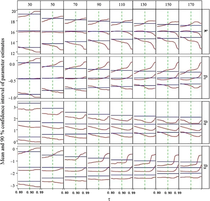
Fig.4 A multi-panel display of mean and 90% confidence limits of 2000 estimates for each of the four parameters of the self-thinning surface estimated through the normal-half normal stochastic frontier model (blue lines) and through quantile regression over 20 evenly spaced σ values from 0.80 to 0.99 (red curves) across the eight sample sizes as denoted in the top stripe of each column

Fig.6 Multi-panel display of the skewness of the 2000 estimates for each of the four parameters of the self-thinning surface estimated through the normal-half normal stochastic frontier model (blue lines)and through quantile regression over 20 evenly spaced σ values from 0.80 to 0.99 (red curves) across the eight sample sizes as denoted in the top stripe of each column

Across all eight sample sizes and over the quantile range of 0.90 ≤σ≤0.99 that is most applicable for estimating the self-thinning surface in higher dimensions,the normal-half normal stochastic frontier model proved to be superior to quantile regression in the sense of statistical efficiency.Its parameter estimates had much lower degrees of variability and correspondingly narrower confidence intervals (Figs.4,5).This greater efficiency would naturally be conducive to detecting differences among species,forest types,site classes and other environmental and climatic conditions through statistical inferences.When the entire data set of all 170 observations were used in the estimation,the model had only six positive residuals and therefore the estimated self-thinning surface enveloped about 96.5% of the data points.This degree of envelopment would be equivalent to a regression quantile estimation with aσof 0.965,but it was achieved with a much greater degree of precision through the stochastic frontier estimation.Such comparative performances of the two methods could also be seen from the results reported but not noted or elaborated by Zhang et al.(2013).Furthermore,the stochastic frontier estimation could lead to a more objective self-thinning surface because it did not involve the subjective selection of a particular value ofσto peel through the data space in high dimensions as in quantile regression.

However,quantile regression could still provide a valuable complement to stochastic frontier analysis in the estimation of the self-thinning surface as it allowed the examination of the impact of variables other than stand density,namely S and W in this case,on different quantiles of stand biomass.The quantile regression estimates ofβ2andβ3,the two parameters associated with relative site productivity S and the abundance of woody weeds,exhibited somewhat different patterns of quantile-dependence(Table 3,Fig.4).Whenσincreased from 0.80 to 0.95,generally decreased butshowed no obvious change trend.Asσfurther increased,bothandincreased,but with the former less so than the latter.The effect of site productivity and the impact of the abundance of woody weeds on the accumulation of stand biomass were not the same across the conditional quantiles.Such differences,when carefully examined,would provide a greater insight into the growth dynamics of the even-aged larch stands growing under the self-thinning surface.This complementarity between stochastic frontier analysis and quantile regression argues for the application of both methods in the estimation of the self-thinning surface in high dimensions,especially when dealing with data that do not conform to the distributional assumptions of stochastic frontier models.

Conclusions

For estimating the self-thinning surface in higher dimensions using cross-sectional data,the normal-half normal (NH)stochastic frontier model proved to be superior to quantile regression over the quantile range of 0.90 ≤σ≤0.99 across small as well as large sample sizes.The superiority lies not only in the statistical efficiency of parameter estimation but also in the greater objectivity of the stochastic frontier model as it does not involve the subjective selection of a particular value ofσas in quantile regression.The higher statistical efficiency and greater degree of objectivity are conducive to making statistical inferences about the parameters of the self-thinning surface.However,quantile regression can still provide a valuable complement to stochastic frontier analysis in the estimation of the self-thinning surface because it can deal with data that do not conform to the distributional assumptions of stochastic frontier models and help reveal the impact of variables other than stand density on stand biomass at levels ofσbelow the estimated surface.

AcknowledgementsWe are indebted to the academic staff,and past and present postgraduate students of the Department of Forest Management,School of Forestry,Northeast Forestry University,who collected the field data.

Open AccessThis article is licensed under a Creative Commons Attribution 4.0 International License,which permits use,sharing,adaptation,distribution and reproduction in any medium or format,as long as you give appropriate credit to the original author(s) and the source,provide a link to the Creative Commons licence,and indicate if changes were made.The images or other third party material in this article are included in the article’s Creative Commons licence,unless indicated otherwise in a credit line to the material.If material is not included in the article’s Creative Commons licence and your intended use is not permitted by statutory regulation or exceeds the permitted use,you will need to obtain permission directly from the copyright holder.To view a copy of this licence,visit http://creat iveco mmons.org/licen ses/by/4.0/.