The Numerical Solution of 3D Free Surface Wave for Double Hydrofoils

ZHAO Le-ping, LUO Zhi-qiang

(1- School of Science, Kunming University of Science and Technology, Kunming 650500;2- School of Media Engineering, Zhejiang University of Communication, Hangzhou 310018)

Abstract: In this paper, a source panel method with dissipative Green function is applied to explore the internal evolution mechanisms under the interaction between the complicated 3D flow field and double hydrofoils. Based on the dissipative source Green function, the different wave profiles of free surface are presented in the double hydrofoils flow. From the benchmark tests, we can draw a conclusion that the accuracy and robustness of the numerical algorithm can be confirmed. Numerical results show that the evolution of wave profile of single hydrofoil and double hydrofoils can be demonstrated clearly. The parallel wave ripple will interact with the other waves and the crest and trough can be overlapped. The double hydrofoils systems can present different wave ripple profiles obviously corresponding with the different staggered position.

Keywords: potential flow; dissipative Green function; singular wave integral; second Green’s formula

1 Introduction

The numerical solutions of 3D potential flow with respect to a hydrofoil beneath the free surface are well known. Most of the published papers on the wave-body problem are about approximate solutions. The wave integral expression of the 3D Green function is too complicated to be expressed in the form of elementary functions. So its efficient numerical calculations have been important in ship hydrodynamics. These problems have been discussed by[1—5]. Schwartz[6]formulated the boundary-integral technique in an inverse plane. Thereafter,Stoker[7],Coleman[8]and Caoet al[9]considered numerical solutions for three dimensional nonlinear free surface. Iwashita and Ohkusu[10], Yanget al[11], Peter and Meylan[12]studied the Green function to simulate all kinds of wave elevations. Some approximate techniques [13—15] were presented in order to calculate the Green function. Wuet al[16]presented a practical analytical approximation of the steady linear potential flow around a ship’s hull. Shanet al[17]investigated the new implementations of efficient approximations of Green function.

In order to avoid the singular integral and computation divergence, we apply an energy dissipative approximation technique to calculate the double hydrofoils system.Based on the research of the dissipative vortex Green function in Chen[13]that is suitable for a single hydrofoil, we study the dissipative source Green function that is suitable for double hydrofoils and apply it to simulate free surface wave elevation with different dissipative parameters, water depth and velocity in the uniform flow.

2 Physical model

Consider an incompressible, irrotational and inviscid liquid with infinite depth.The fluid domain possesses an upper free boundary and is subject to the downward acceleration g of gravity. A Cartesian coordinate system is defined such that thez-axis points vertically upwards, and thexandyaxes lie in the plane of the undisturbed free surface, as show in Figure 1. The single hydrofoil and double hydrofoils are submerged beneath the fluid with the vertical distancehmeasured from the undisturbed free surface to the hydrofoils.

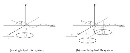
Figure 1 Physical domain

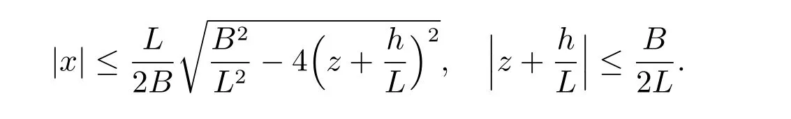
The size of the hydrofoil is similar to an ellipse, together with the lengthLand the diameterB. The wave elevationηcan be measured, which is the distance from the undisturbed free surface to the free surface. The single thin spheroidSis defined byy=±f(x,z). The double spheroids are defined byf1(x,z) =c ± f(x,z) andf2(x,z) =-c±f(x,z),cis the horizontal distance measured from thezaxis to the center of the spheroid. Here, the functionfis denoted as

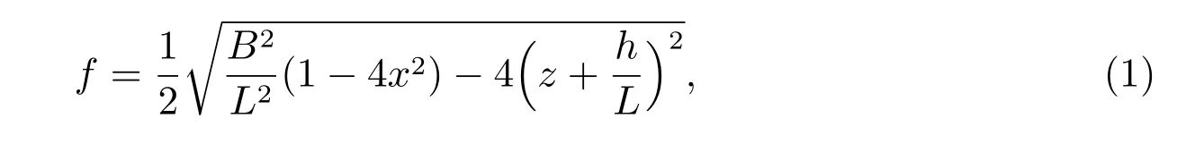
for

3 Control equations

The total velocity potential Φ of the fluid domain is denoted by the equation

whereφ*is the perturbed velocity potential of the fluid.Uis the horizontal velocity of uniform fluid along thex*positive direction.

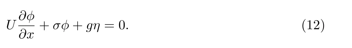
The linear Bernoulli equation on the free surface is given by the equation

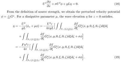
whereμ*is a dissipative parameter on the free surface.

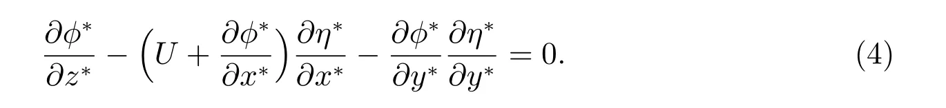
The kinematic boundary condition on the free surface is given by the equation

The wave elevation on the free surface is given by the equation

We give the following dimensionless formulations

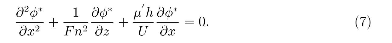
By the linearized method, the equations (3) and (5) can be simplified to the following formula forz=0

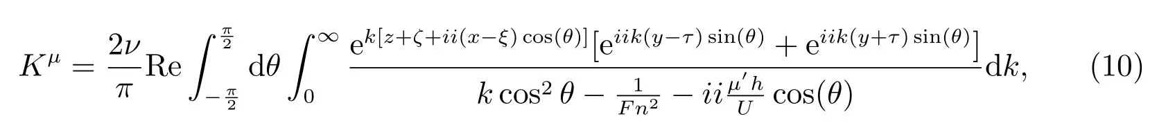
A source of constant strength in an uniform fluid is submerged beneath the free surface.The source lies in the location with the coordinate (ξ,τ,ζ),ζ ＜0. The Green functionGis represented from the Havelock and the formula is based on a plane Fourier transformation. The complicated Green functionGμis a superposition of the Rankine source potential given by the equation

whereKμsatisfies the boundary condition (7).

Observing that

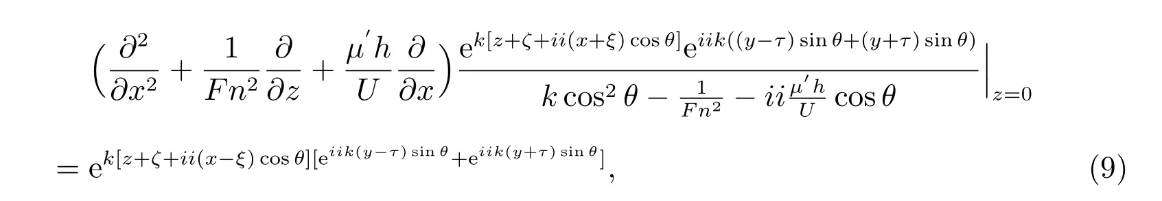
we can choose the Green function

whereμ′is known as Rayleigh’s artificial viscosity coefficient, and ΔKμ= 0. In particular,iiis used to denote the imaginary unit in this paper.

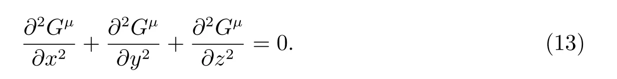
The velocity potential satisfies the Laplace equation

and the linearized Bernoulli equation is rewritten by

The Green function satisfies the Laplace equation

Due to this fact, which the Green functionGμand velocity potentialφsatisfy the boundary integral equation, we can derive the boundary integral equation

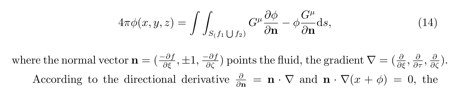
From the linearized dissipative Bernoulli equation, the dimensionless form is denoted as

4 Discretization of dissipative Green functions

Substituting the equation (10) into the equation (19), we get this formula

The discretization of the boundary integral equation is presented with the mesh grid points (ki,θj) withi= 1,2,··· ,N1+1 andj= 1,2,··· ,N2+1 in the integral equation. In addition to that the projection domain is discretized by the mesh grid points(ξn,ζm), n= 1,2,··· ,N3+1 andm= 1,2,··· ,N4+1. The equation (20) can be rewritten as the following integral approximation

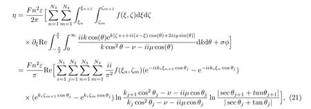
forσ=0.

5 Numerical results

5.1 Benchmark test

In this section, in order to validate the accuracy and robustness of the proposed algorithm, two tests are presented and compared with previously published papers.

The parameters are selected withh=-1, μ= 0.001, ϵ= 2.6 andFn= 0.7.Lis the typical length in the fluid domain. The convergence study is presented in Figure 2. The circle line corresponds to the results in Tuck and Scullen[4], and the solid line is the present solution. From Figure 2,the current numerical results are highly coincident with the results of paper [4].

Figure 2 3D free surface wave for y =0, μ=0.001, ϵ=2.6 and Fn =0.7

The second benchmark test is to validate the sensitivity of numerical solutions with respect to different dissipative parametersμ. In Figure 3, the wave elevation on the free surface is calculated with respect to a uniform flow passing a submerged spheroid.As shown in the picture, the numerical solution of the wave elevation has no sensitive dependence on the small dissipative parameterμ. We can draw a conclusion that the error between the dissipative Green functionμ=0.001 and the singular wave integralμ=0 can be ignored.

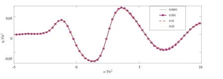
Figure 3 3D free surface wave for y =0, ϵ=2.6 and Fn =0.45

5.2 Numerical simulation

After the above numerical validation, the developed numerical model is used to analyze the 3D wave elevation in a uniform fluid passing a single or double hydrofoil model. In the following subsections, we will discuss the wave elevation of a single hydrofoil system, when the parameterτ=0.

The parameters are selected ash=B, μ= 0.001, ϵ= 2.6, c= 0 andFn= 0.6.In Figure 4, the numerical solution of the 3D wave elevation is simulated for a single hydrofoil system. We can clearly see the 3D wave with respect to the uniform flow passing the submerged spheroid. And the 3D wave spread backward as transverse waves.

The double hydrofoils are rarely used to calculate the numerical solution of the 3D wave. The parameters are selected byh=B, μ=0.001, ϵ=2.6, c=handFn=0.6.As shown in Figure 5, we present the wave profile for the parallel double hydrofoils system and the free surface wave of ship can be seen clearly. In order to investigate the evaluation of flow wave, the double hydrofoils must be established with different locations. The double hydrofoils can be arranged in alphabetical order and we can see a different profile. The wave profile is partially reduplicated in Figure 6. In Figure 7,the double hydrofoils are arranged parallelly and tilted,we can see another scene of the 3D wave elevation.

Figure 4 3D free surface wave for y =0, ϵ=2.6 and Fn =0.6

Figure 5 3D free surface wave for paratactic double hydrofoils

Figure 6 3D free surface wave for tandem-double hydrofoils

Figure 7 3D free surface wave for tandem-double hydrofoils

6 Conclusion

A new algorithm of the dissipative Green function is developed with respect to single hydrofoil and double hydrofoils in a potential flow. Numerical experiments show that the developed numerical model is used to analyze the 3D wave elevation of uniform fluid passing through single or double hydrofoil models. From the Figure 4 to Figure 7 show the numerical solutions of 3D free surface wave elevation. Due to hydrofoils interfere with each other, the wave crests and troughs overlap each other, and spread backward as transverse waves. The double hydrofoils systems can present different wave ripple profiles obviously with respect to the different staggered position.