Bivariate joint distribution analysis of the flood characteristics under semiparametric copula distribution framework for the Kelantan River basin in Malaysia

Shahid Latif ,Firuza Mustafa

Department of Geography,University of Malaya,Kuala Lumpur 50603,Malaysia

Abstract Flood is becoming the severe hydrologic issue at the Kelantan River basin in Malaysia.The joint distribution analysis amongst multiple interacting flood characteristics,i.e.,flood peak discharge flow,volume,and duration series usually provide a comprehensive understanding of the hydrologic risk assessments through visualizing the multivariate exceedance probability or return periods.The traditional copulas-based methodology is frequently employed under parametric settings where parametric family functions are often employed to model univariate marginal distribution before capturing their dependence structure.Actually,no universal rules and literature are imposed to model any flood vectors through any fixed or predefined density function,which would follow the different distribution and needs to model by fitting most parsimonious function.Also,the copula function already relaxes the restriction of selecting marginal distributions from the same distribution families.Therefore,incorporation of non-parametric kernel density estimations or KDE would be much stable and less biased smoothing alternatives than the parametric approach.In this literature,the semi-parametric copula-based methodology is incorporated,where the flood marginals are modelled under the kernel functions and applied as a case study for 50 years annual maximum (AM) flood samples of the Kelantan River basin at the Gulliemard Bridge gauge station in Malaysia.The Archimedean families copulas (i.e.,Frank,Gumbel and Clayton) and Elliptical copula (i.e.,Gaussian copula) are tested,and thus best-fitted copulas are employed to model the bivariate joint distribution amongst flood characteristics,and which further employed to derive joint and conditional return periods.

Keywords: Flood;Kelantan River basin;Semiparametric Copulas framework;Nonparametric marginal distribution;Kernel density estimation;Return periods.

1.Introduction

Basin perspective water-related issues often demand the accurate estimations of flow exceedance probability for assessing flood risk [1,6,14,55,28,53].Flood is a multivariate stochastic phenomenon usually characterized thoroughly through its mutually correlated vector,i.e.,flood peak discharge flow,volume and duration of flood hydrograph [78,79].Statistically,the flood frequency analysis or FFA is an approach to relate the strength of flood quantiles to their frequency of occurrence by fitting most logical probability distribution functions [56,75].Establishment of the univariate FFA or return periods using the one-dimensional probability functions would be problematic,which might reveal for the underestimation (or risk of failure due to low design value)or overestimation (or the higher cost in hydraulic constructions) of the associated risk of correlated flood characteristics,thus often demands multivariate analysis amongst the mutually correlated flood characteristics and estimating the design variable quantiles under the different notation of return periods,i.e.,based on joint distribution,conditional distribution or Kendall’s distribution (or survival function) [76,65].The multivariate flood analysis often provides a full screen or prediction of hydrologic risk based on the joint probability density functions or PDFs and joint cumulative distribution functions or CDFs.Also,no one could deny from the facts that the potential damage could likely be a function of several inter-correlated flood characteristics.Thus ignorance of spatial dependencies amongst these flood vectors would be revealed for underestimation of uncertainty distributed over the estimated design quantiles,therefore,demands for the accountability of more flood vectors [60,33].

The necessity of estimating design hydrograph instead of just estimating the flood quantiles derived from single variable such as either flood peak /or volume /or duration motivated numerous literature towards the incorporation of the distinct varieties of traditional bivariate or trivariate distributions for establishing the mutual dependencies amongst flood characteristics [39,10,24,77,75,26].All the above multivariate approach often surrounded with several statistical limitations such as;(1) each flood vectors must assume to have Gaussian or normal distributions or either transformed to have normal distributions;(2) the statistical parameter of the univariate marginal structure is often employed to model their joint dependence structure;(3) the availability of limited space to justify the joint dependence structure under traditional multivariate functions,[78,79,62,63].In actual,each induvial hydrological vector would be following different marginal structure and desire to model separately using the best-fitted distribution functions independently from their joint structure.De Michele and Salvadori [23]firstly incorporated the copulas function for establishing joint structure between storm intensity and duration samples.In actuality,the copulas function is recognized as a highly flexible multivariate tool which segregated the modelling of univariate vectors and their joint dependence structure separately into two distinct stages [72,70,51].Copulas usually attribute for higher flexibility in the selection of best-fitted marginal distributions and their joint structure to capture a more extensive extent of mutual concurrency and preservation in their joint association.Genest and Favre[81]provided an extensive review of the application of copulas in the field of engineering and sciences.Besides this,extensive literature incorporated bivariate or trivariate copulas distribution as a model risk such as,for flood modelling[12,21,28,53,65,70,87],drought modelling [63,4]rainfall or storm modelling [66,41]or either modelling of hydro-climatic series [19,22].

In the above-cited literature,the copula-based methodology is frequently incorporated under the parametric settings,where the parametric family functions are frequently employed to modelled univariate marginal distributions also,the parametric copula function for establishing joint dependence structure (i.e.,[65,56,28]and references therein).However,the parametric functions always imposed an assumption that random samples are coming from the known populations whose PDF are pre-defined or assumed to follow some specific family of parametric density functions [37].No universal rules and literature are imposed to model any hydrologic or flood vectors through any fixed or pre-defined distribution functions,which would follow different distributions and desire to model separately or in other words,the best-fitted marginal distributions are not from the same probability distribution family [2,74,76,40,9].Also,according to Dooge [20],it is already pointed out that no amount of statistical refinement can overcome the consequences due to the lack of prior distribution information of the observed random samples.Also,it would be not easy to approximate distribution tail beyond the most significant values under the parametric distribution framework [13].Therefore,in the past few decades,an attempt via kernel density estimators or KDE is recognized as a much flexible and stable nonparametric data smoothing procedure to inference about the populations based on finite observational samples and thus motivated in the field of hydrologic or flood frequency analysis and which often yielding a bonafide density function [2,1,5,6,46,8,67,27,44,45,37,69].Nonparametric marginal distribution did not require any prior distribution assumptions and will be directly retrieved from distributed series with a greater extent of flexibility in their univariate function as compared with parametric density estimators [1,48].

The parametric copula distribution framework often depends upon the prior knowledge of the univariate marginal distribution function as well as the joint distribution function.However,on the other side,the copula modelling already relaxes the restriction of selecting marginal distributions from the same distribution families.According to Choros et al.,[18]and Srinivas and Santhosh [69],the copula modelling can be categorized as parametric,semiparametric and nonparametric,which solely depends upon the procedure in which their univariate marginal distribution and joint dependence structure are estimated.Such that,in the parametric copula framework,the univariate marginal distribution of individual random characteristics and approximation of their joint dependence structure is carried out using the parametric settings (i.e.,the parametric family based univariate probability distribution as well as parametric copula function.Similarly,in the semiparametric copula distribution framework,the marginal distribution of univariate characteristics is approximated using the nonparametric distribution fitting procedure (i.e.,KDE).However,their joint dependence structure is still modelled with parametric copula settings (i.e.,parametric copula families function like the Archimedean copulas or Elliptical copulas).On the other side,in the nonparametric copula distribution framework,both their univariate marginal distributions as well as mutual dependency are modelled using the nonparametric distribution procedure.Literature such as Rauf and Zeephongsekul [57]demonstrated through the incorporation of nonparametric copula distribution approach for the rainfall characteristics and thus revealed that the nonparametric approach can often give better results than a purely parametric approach.It is already discussed in the above paragraph that in the multivariate hydrologic data analysis,parametric copula-based methodology frequently appears in the literature,on another side,some literature motivated towards the semiparametric copulas procedure (i.e.,[38,56]).Similarly,literature such as Harrell and Davis [35],Brown and Chen [15],Chen [17],Bounezmarni and Rombouts [84],pointed the importance of nonparametric copula distribution framework,also called the Beta kernel copula density function.Most of the earlier demonstrations introduced parametric function for defining the marginal distribution of flood peak,volume or duration samples (i.e.,[70,21,79]and reference therein).Therefore,in such circumstances,how one could significantly enjoy the flexibility or efficacy of copula functions in conjunction with the nonparametric marginal structure in the modelling of flood characteristics.Karmakar and Simonovic [37],introduced the bivariate parametric copulas in the establishment of flood dependence structure with mixed marginal distributions,also called heterogeneous marginal environment.In this experiment,both the nonparametric based on kernel density function and the orthonormal series,as well as the parametric functions,are tested for defining most appropriate marginal distribution functions.Similarly,Reddy and Ganguli [56],modelled the flood characteristics using bivariate copula functions where the nonparametric based on kernel density estimators recognized as a best fitted marginal distribution for most of the flood vectors along with parametric families of distribution.

The Kelantan River basin is often subject to the most severe monsoonal flooding in Malaysia and perceiving for increasing in term of their frequency and magnitude [7].It is one of the largest basins in Malaysia known to be flood-prone.The maximum length and breadth of this catchment area are 150 km and 140 km,respectively,and about 248 km long and drains an area of 13,100 km2,occupying more than 85% of the State of Kelantan.The intense and prolonged precipitation in the year 2002 caused flooding of a total area of 1640 km2and affected the population of 714 287.Similarly,in the early month of December 2014,much heavy precipitation occurred for many of days triggered the flood event in the several parts of the east coast of the Kelantan river basin,and it was the worst flood ever recorded in history and affected more than 20,0000 people [7,59].The cause of frequent failures of flood defence infrastructure in Malaysia due to the impact of moderately severe of flood episodes might be responsible due to the lack of complete flood hydrograph or in other words,where only flood peak discharge samples often targeted in deriving flood frequency curve during the structural development.Therefore,multivariate probabilistic assessments of flood characteristics and their associated return periods could be a comprehensive way for making a defensive risk-based decision making in the various basin perspective water-related issues.This study incorporated the semi-parametric copulasbased methodology for establishing the bivariate joint distribution relationship of the flood characteristics,i.e.,flood peak discharge flow (P),volume (V) and duration (D) series.The probabilistic model has implemented on the block(annual) maxima based flood sampling procedure in which the daily basis streamflow discharge records from the period 1961-2016 are collected in the Kelantan River Basin at the Gulliemard Bridge gauge station in Malaysia.The nonparametric statistical framework is selected where an interactive set of univariate kernel density functions is tested for approximating the marginal distribution of individual flood characteristics.After that,the efficacy of 2-dimensional parametric copulas family is tested to construct a bivariate joint relationship between flood characteristics under the nonparametricmarginal environment.Finally,the best-fitted bivariate copulas,along with the nonparametric marginal distribution are employed to derive the joint and conditional return periods.

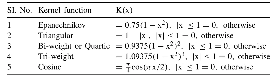
Table1 Some standard univariate kernel distribution functions.

2.Theoretical framework

2.1.Nonparametric estimates of univariate marginal distribution

The concept and idea of the kernel density estimators or KDE are firstly introduced by the Rosenblatt [61],it is a way of smoothing kernel weights on each of the random observations.It is a nonparametric approach to approximate the probability density functions or PDF of given random observations or say flood vectors such as flood peak flow,volume and durations.Mathematically,the univariate kernel functions are used to estimate the probability density of the random observations having the following statistical property as given below:

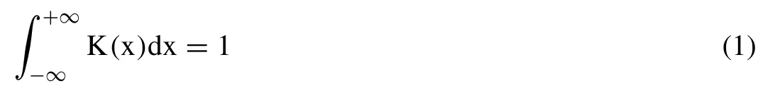
where ‘K (x)’ is defining the univariate kernel function,which can be employed as a density function or PDF [37],however,one can easily approximate the kernel functions through the general equation (i.e.,[34]) as given below:

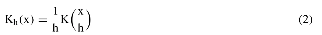
where ‘h’ is called the smoothing parameters called bandwidth of Kernel functions.Kernel bandwidth can be used for regulating the level of smoothness and roughness in the shape of estimated PDF [48].Mathematically,one can easily retrieve the univariate Kernel density estimates of a random observation say X1,X2,X3,....Xnand having PDF,f(x)by averaging the Eq.(2) in the given random samples are as given below [50,40]:

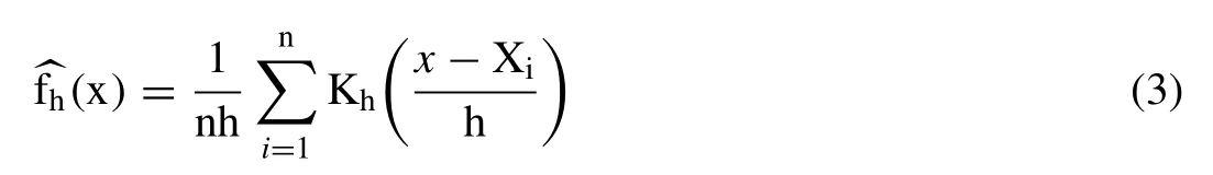
where ‘n’ is the number of random observations;Xiis the ithobservations andis the kernel density estimates.The efficiency of the estimated kernel density function depends upon two factors;(1) an appropriate choice of the kernel bandwidth and (2) the selection of kernel functions considered for estimations.Table1 listed some of the standard univariate kernel functions and their mathematical relationships,suchas Epanechnikov,Biweight,Triweight,Cosine and Triangular kernel function,which are incorporated in this literature for determining the density function or PDFs and cumulative function or CDFs and assigning appropriate marginal distributions of each individual flood vector (i.e.,Moon and Lall;[50,37]).According to Epanechnikov [25],the Epanechnikov kernel function is optimal in a mean square error sense.Kernel functions listed in Table1 are ideally suited for unbounded observations,but in actuality,most of the hydrologic data like rainfall,streamflow or humidity is either upper or lower side bounded and attributed to the boundary leakage problem.Method of reflection [74]&[106],Methods of transformations [49],Beta kernels [17],Adaptive kernels [9]are several approaches to tackle such issues.

Table2 Bandwidth estimation algorithms in the kernel density estimation.

An appropriate choice of the kernel smoothing parameter or bandwidth ‘h’ is often a significant concern that controls the shape of kernel density estimates [47,27,40].The insufficient or over smoothing would result for rough density or bypass away from the critical feature [69].Table2 summarizes different bandwidth selection algorithm such as Rule of Thumb (ROT) (i.e.,[74]),Least-squares cross-validation(LSCV) approach (i.e.,Tarboton et al.,1998),Bandwidth factorized cross-validation approach (i.e.,[40]),Smoothed crossvalidation approach (i.e.,Hall 1992),Biased cross-validation approach (i.e.,Scott and Terrell 1987),Maximum likelihood cross-validation (MLCV) approach (i.e.,[86]),Plug-in estimates approach (i.e.,Wand and Jones 1995) and Asymptotic mean integrated squared error (AMISE) approach (i.e.,Ghosh and Huang 1992).Besides this,Jones et al.,[36]and Sharma et al.,[67]provided an extensive overview of this algorithm and their approaches in kernel estimates.The several bandwidth estimation procedures are solely based on minimizing the estimates of the Mean square error or MSE [68]which means it is usually estimated by reducing the gap between theoretical pdf and the actual one.The asymptotic mean integrated square error or AMISE depends on kernel bandwidth,kernel function,sample observations size and targeted density functions [50].Therefore,by selecting an appropriate kernel function and a kernel bandwidth value,it could be possible to minimize AMISE value.According to Silverman[74],the rule of thumb or ROT is proposed to minimize the asymptotic MISE value.Therefore,Azzalini [3]and Silverman [74]demonstrations estimated the optimal bandwidth h0,which is based on the fact that the final distribution to be Gaussian or symmetrical and can be formulated as:

where,′σ′is the minimum {Sample standard deviation,(Interquartile range or IQR/1.349)}.In the present demonstration,the bandwidth of the kernel density functions is estimated using Eq.(4).

2.2.Multivariate copulas function

The ideas and concept of the copula function have been developed by Saklar [72].The copulas connect multivariate probability distributions to their univariate marginal probability distribution functions ([52],2006).According to Sklar’s theorem [51],if (X,Y) be the bivariate random variables with continuous marginal distributions,u=FX(x)=P(X ≤x)andv=FY(y)=P(Y ≤y)then it can be characterized uniquely by its associated dependence function called Copula or C which can be defined on the unit square,can be expressed as:

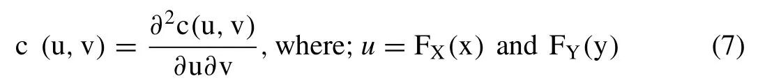
where,‘C’ is any type of bivariate copulas under consideration;FX(x)=FY(y)is the cumulative distribution functions of univariate random variables say ‘X’ and ‘Y’;HXY(x,y)is the bivariate joint distribution functions which can be expressed in terms of the univariate marginal functions and the associated dependence function C.The copula C must be unique if FX(x)and FY(y)are continuous,which can easily capture the wider extent of dependencies amongst random vectors [64,79].Conversely,Eq.(6) must defines the bivariate joint distribution structure between univariate marginal distribution FX(x)and FY(y),if FX(x)FY(y)and copula C(x,y)is given.On the other hand,if fX(x)and fY(y)are the pdf of random variable say X and Y,then the joint probability density of the two random variables can be expressed as:

where,‘c’ is the density function of bivariate copula C,which can be derived using the following relationship as given below:

For the extended mathematical details about copula functions,readers are advised to follow the following pieces of literature,i.e.,Genest and Rivest [31],Nelsen [52]and Nelsen[51].

Interactive sets of copula function are often incorporated in the bivariate dependency modelling of hydrologic extremes such as the Extreme value class (i.e.Gumbel-Hougaard or GH,Galambos &Husler-Reiss),Elliptical class (i.e.Gaussian family),unclassified Plackett &Farlie-Gumbel-Morgenstern (or FGM) parametric functions and three-parametric Twan family (i.e.,belong to the extreme value class).The Archimedean class copulas (i.e.,Ali-Mikhail or A-M-H family,Frank family,Clayton or Cook- Johnson(C-J) family and Gumbel-Hougaard (G-H) family) have frequently accepted due to its vast varieties of families and also its capability to capture the mutual dependencies for a more extensive extent ([23,70,29,51,79,71]references therein).In this study,we introduced and tested several bivariate copulas such as one elliptical family,i.e.,the Gaussian copula,and the mono-parametric version of Archimedean families,i.e.,Clayton,Gumbel and Frank copulas for establishing the bivariate joint dependency of the annual basis flood characteristics,flood peak flow,volume and duration series under the semiparametric copula distribution framework.Mathematically,the copula function (i.e.,[C: [0,1]2 -→ [0,1]]) approximate the bivariate Archimedean class copula if it justify the representation,as given below:

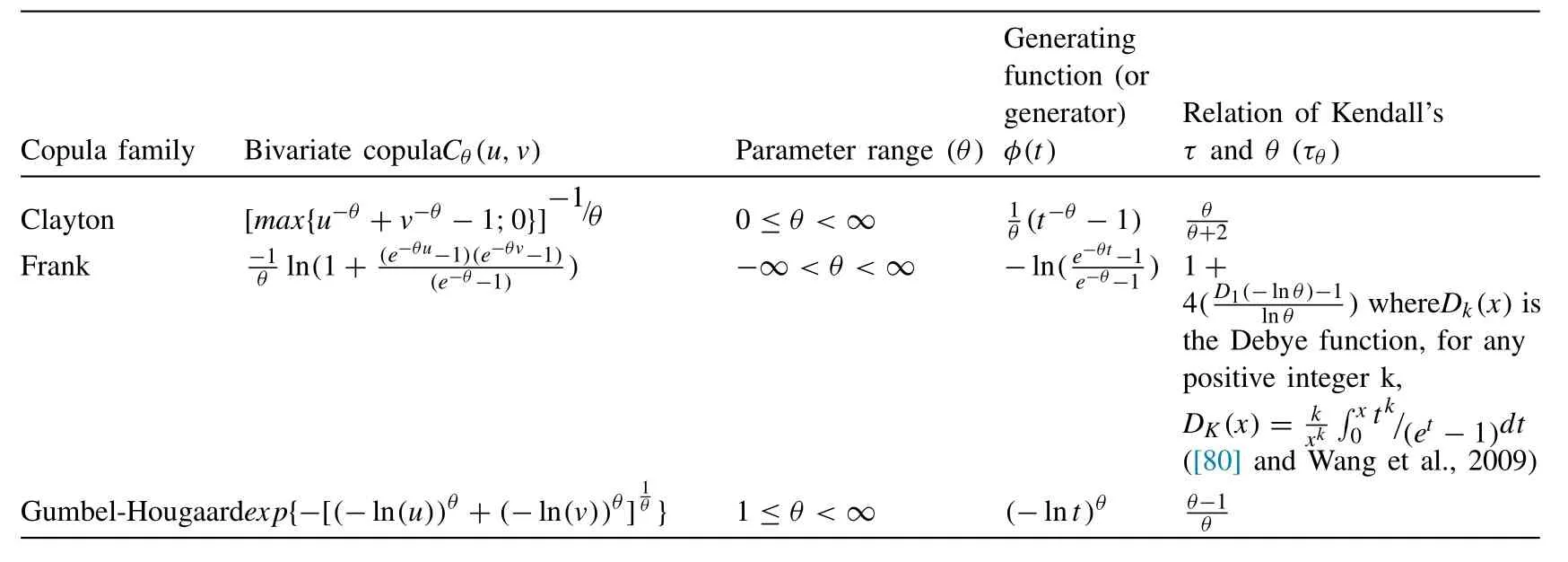
Table3 Mathematical expressions for the bivariate Archimedean copulas and their associated properties (i.e.,parameter range,generating function and Relationship between Kendall’s τ and θ (τθ)).

where,(Ø (.) &Ø-1) is the generator function of the specified Archimedean copulas and their inverse such that the generator (φ: I -→R+) signifies for the positive,convex and decreasing function and could be approximated for (Ø (1)=0&Ø (1)=∞) [51,56].The extent of the dependency capturing capability of each family of Archimedean class copulas is different and which is constrained by the degree of interassociation or dependency measures between random vectors.The Clayton and Gumbel family copulas are only significant to capture positive dependency and having Kendall’s tau range isτθ≥0 ([70,51];Xu et al.,2015).The Frank family function exhibited higher versatility due to its capability in accommodating and capturing the entire range of dependencies (i.e.,τθ∈ [1,-1]) and only member that justified radial symmetry as well (i.e.,symmetric tou+v=1) [23,29,51,80].Except the Frank copula exhibited non-symmetrical behaviour concerning secondary diagonals,all the remaining Archimedean copulas such as G-H copula is much suitable to model upper-tails dependency and Clayton copula exhibited strong capability to model with lower tail dependency.In contrast,Frank copula has no tail dependency [54].Table3 illustrated the mathematical expression (i.e.,the range of its dependence parameters,generating functions or generator and relationship between Kendall’s tau andτandθ,also calledτθ)for the bivariate Archimedean copula functions such as the Clayton,Frank and Gumble-Houggard copula.

On the other side,the Elliptical family-based Gaussian copula is also introduced as a candidate model for testing their adequacy in the establishment of bivariate joint dependency simulations of the flood characteristics.The Gaussian copula shows almost no dependence in the tails and is mostly distributed around the centre of the distribution,but because of simple intuition as it is based on the normal distribution,it is quite popular amongst the hydrologist and water practioner in extreme event modelling ([115];Kamaruzaman et al.,2018;[16]).The Gaussian copula is an implicit copula,which can be expressed as an integral over the density of X,can be expressed mathematically in the bivariate case as given below([116]):

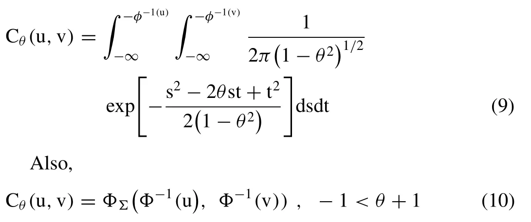
Where′Φ′is the cumulative distribution function of standard normal or Gaussian distribution.

2.3.Estimation of copulas dependence parameter

According to [91],the different approach of the copula parameter estimation can be classified into two main groups,such as the ranked based procedure and the other methods.The method of moment (MOM) which is based on the ranked based non- parametric measures such as Kendall’s tau (τ) or Spearman’s rho (ρ) (i.e.,[31,56]a),exact maximum likelihood or EML (i.e.,Zhang et al.,2016),inference functions for marginal or IFM (i.e.,[99]and [29]),canonical maximum likelihood or CML [95],Maximum pseudolikelihood estimations (MPL) (Genest et al.,1995) are some popular algorithms,widely accepted in the estimation of copula dependence parameters.In this literature,MPL estimator is incorporated for the estimation of the copula dependence parameters.The MPL estimator is a modified version of the traditional maximum likelihood method where the rank based empirical distributions are used and can be applied for both the one or multi-parameter copula functions.MPL parameter estimates are widely accepted by many authors (i.e.,[21,101,42,56]) because the copula dependence parameters are usually estimated independently from their univariate marginal distribution functions.Based on maximizing the pseudo-log-likelihood function,one can easily estimate the copulas parameter,can be expressed as:

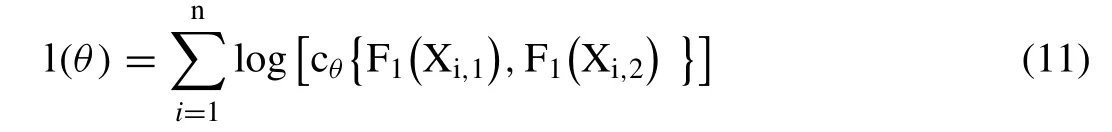
where,′θ′is the copula parameter;l(θ)is the pseudo loglikelihood function;F1(Xi,1)=F1(Xi,2)defines the empirical CDFs.

2.4.Testing the fitness level fitted bivariate copulas

In this demonstration,the Cramer-von Mises test statistics are employed to evaluate the adequacy of hypothesized copulas fitted to bivariate flood characteristics,and it’s often considered as one of the most powerful tools for investigating the compatibility of the fitted copulas [30,32].This test is based on the parametric bootstrapping procedure that makes the use of the Cramer-von Mises statistic Sn,and can be computed mathematically,as given below [32]:

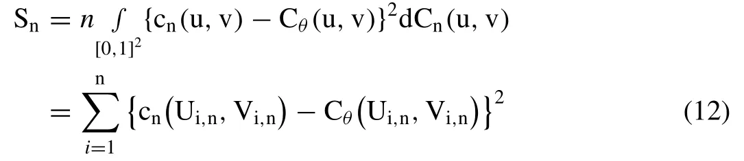
where,′Cn′is the empirical copula estimated using the ‘n’observational flood attribute pairs;′Cθ′is the parametric copula derived under the null hypothesis.There are two different ways to estimatep-value corresponding to the above ‘Sn’test statistics,(1) followed by Genest and Rémillard [30]approach,which is based on via the large simulated samples derived by the mean of the parametric bootstrapping procedure(2) followed by Kojadinovic et al.,[43]and Kojadinovic and Yan [42]procedure which is based on multiplier approach.In this experiment thep-values for each fitted bivariate copulas to observed flood characteristics are estimated using the parametric bootstrapping procedure (i.e.,followed by Genest and Rémillard [30]) and which can be mathematically formulated as given below:

where,‘N’ is the number of simulations.This fitness statistics actually involve the testing of the null hypothesisa gainst the alternate hypothesis′Ha′as given below:

Null hypothesis (H0)=C∈ C0{where,C0=Cθ;θ∈O)

Alternate hypothesis (Ha)=C/∈ C0where,‘O’ is the open subset of ℜqfor some integer value,q.The acceptance or rejection of the considered copulas is based on estimatedp-values.If the estimatedp-value is larger than a significance level,then the null hypothesis must be accepted and which in result,copula must be considered as satisfactory performance otherwise will be liable for rejections.From the Eq.(13),it must be concluded that the minimum value of Sntest statistics must indicate for the minimum gap between empirical and derived parametric copulas.

3.Details of study area and delineation of triplet flood characteristics

The geographical location of the Kelantan River basin is Lat 4 ° 30′N to 6 ° 15′N and Long 101 °E to 102 ° 45′E.It is the longest river in the Kelantan state of length about 248 km long with a total drainage area of 13,100 km2,which is originating from the Tahan mountain range to the South China Sea,in the north-eastern part of Peninsular Malaysia and occupying more than 85% of the state of Kelantan.The estimated runoff of this region is about 500 m3s-1and the variations of annual precipitations are in between 0 mm(dry period) -1750 mm (wet or north-eastern monsoonal period).Literature such as [85,98]and Adnan and Atkinson[7]claimed that due to rapid human intervention from natural to land use activities in the form of deforestations or land clearance which would trigger the risk of such extreme hydrologic happening.This case study is demonstrates for the 50 years (1961-2016) of daily basis streamflow discharge records which are collected and provided by the Drainage and Irrigation Department in Malaysia for the Gulliemard Bridge gauge station,which is located at the downstream of the Kelantan River near the Kuala Kari region in Malaysia.

Annual (Maximum) series or AM also called block (annual) maxima and Peak over Threshold (or POT) are the two holistic techniques which is widely accepted in the extreme probability simulations [93,14,105].In this demonstration,the annual (maxima) series based flood sampling procedure is adopted for constructing the multivariate framework,which often revealing an intuitive procedure for handling complicated hydrological practical (i.e.,[56,73,109]).The partial data series only focuses the extreme hydrograph portion,i.e.,the high flow portion of streamflow characteristics,instead of visualizing entire flood hydrograph ([102];Hosking et al.1985;[14]).Flood peak discharge flow (P),hydrograph volume (V) and duration (D),which are obtained from a daily basis streamflow observations are the main flood vectors in this demonstration.Therefore,the targeted site is characterized by single flood episodes at an annual scale based on their maximum streamflow discharge value and their values are estimated using Eq.(14) (i.e.,[75]).On the other side,the hydrograph volume samples are retrieved corresponding to each annual basis peak series by separating the base flow portion (i.e.,low-frequency components) from the direct runoff portion (i.e.,high-frequency components) called hydrograph volume extraction,and the duration samples are based on thetime difference between the rising (SDi) and recession (EDi)limb of targeted peak curve,followed by Eq.(15) &(16) (i.e.,[76,88]) as given below:

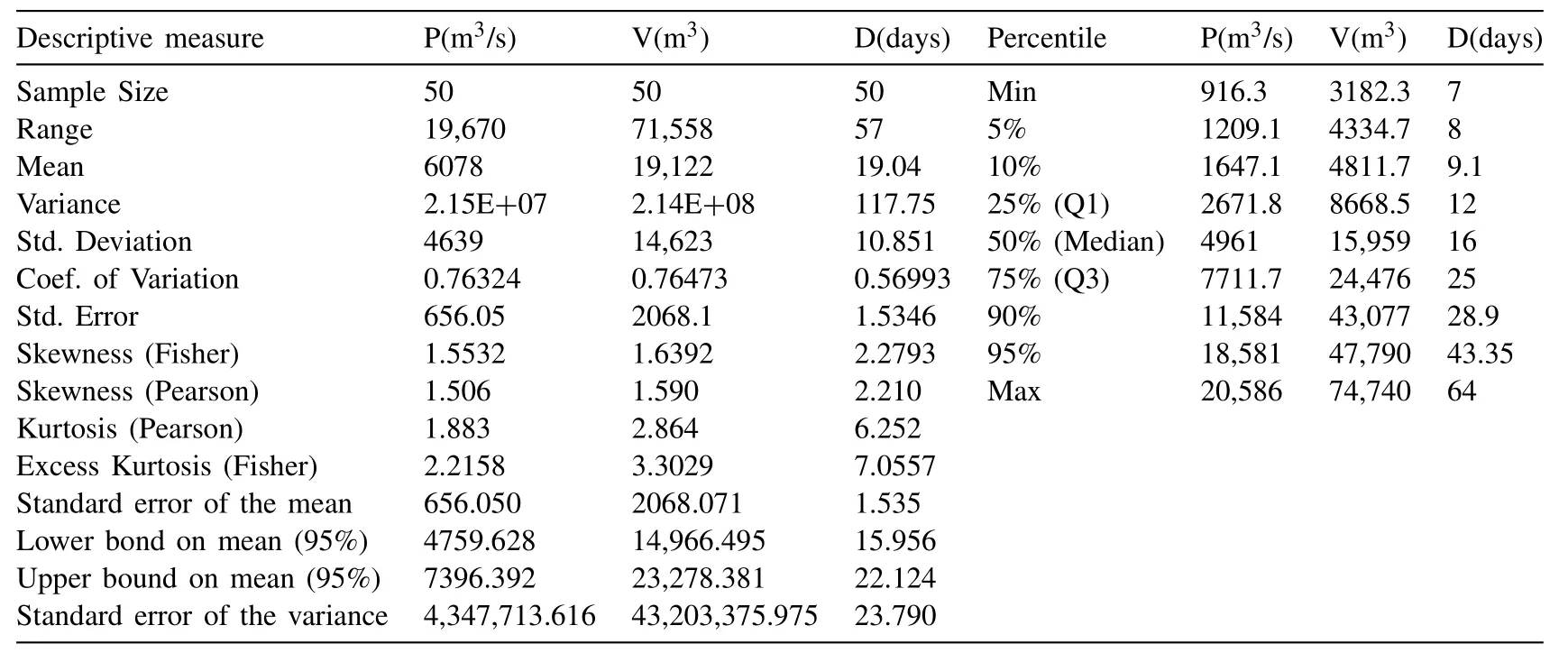
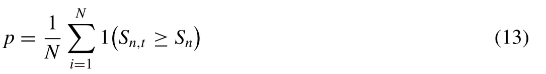
Table4 Descriptive statistics of annual flood characteristics (at the Gulliemard Bridge gauge station).

where′Qij′is the jthdays streamflow magnitude for the ithyear;′Qis′and′Qie′is the streamflow magnitude for the start date′S Di′and end date′ED′iof the flood runoff.It is also pointed that flood peak discharge often attains their maximum value but not mandatory for hydrograph volume &duration series ([73];Xu et al.,2015).

4.Results and discussions

4.1.Approximation of univariate flood marginal distributions

4.1.1.Testforstationaritywithinfloodcharacteristics

The descriptive statistics of the annual flood characteristics for the Kelantan River basin at Gulliemard Bridge gauge station are listed in Table4 and their visual interpretations,via the histogram plot,box-whisker plot and normal quantile or Q-Q plots are illustrated in Fig.2.Selecting the most appropriate univariate probability functions for defining the marginal distributions of each individual flood characteristics is a mandatory pre-requisite desire before introducing the random vector into the multivariate or copulas distribution framework.However,before that,testing the existence of serial correlation or stationary within the individual time series associated with each flood characteristics is also mandatory to ensure whether the flood characteristics are independently distributed or not.A hypothesis testing based on the Q-statistics(i.e.,[104];Daneshkhan et al.,2016) is performed for the different lag size,for investigating whether the individual series are time-independent and having no serial correlation.Statistically,the Q-statistics usually follows a chi-square distribution with ‘h’ degree of freedom under the null hypothesis,H0.Thus,the Q-statistics for the sample size ‘n’ with ‘t’ is the total no of lag being tested with sample autocorrelations at the specific lag size are given below:

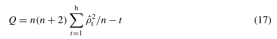
where,Null hypothesis (H0)=zero autocorrelation or independent distributions;and Alternative hypothesis(H1)=existence of serial correlation (or autocorrelation).

The Q-statistics and their associatedp-value for the different lag size (i.e.,20,10 and 5) are listed in Table5 and which revealed the existence of almost zero first-order autocorrelation as their estimated statistics are below their critical value for each of the univariate series of accepting the null hypothesis (H0) at 5% or 0.05 significance level against their alternative hypothesis (Ha).Similarly,the non-parametric rank-based Mann-Kendall (or M-K) test (i.e.,[107];[103]) is also performed for visualizing the monotonic trend and which revealing the existence of zero monotonic trends at the 5% level of significance within time series of individual flood characteristics.The estimated values of M-K test statistics are listed in Table6 and which can be mathematically formulated as:

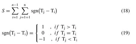
where Tj&Tirepresenting the annual value in year ‘j’ and‘i’,respectively.

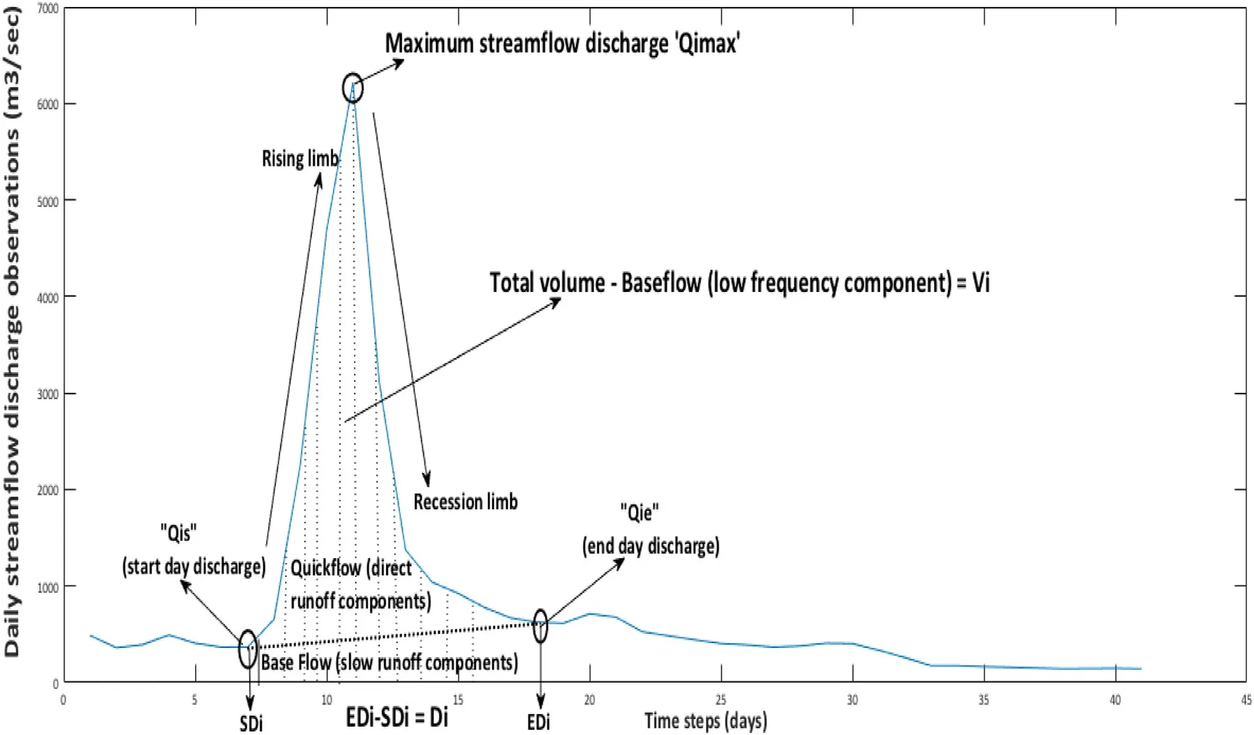
Fig.1.A typical hydrograph characteristic for the i th flood episodes.

Fig.2.Visual interpretation of the flood characteristics in the context of histogram plot,normal Q-Q plot and box-whisker plot.

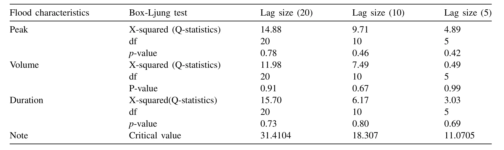
Table5 The Q-statistics and their corresponding p -values for different lag size of annual flood characteristics.

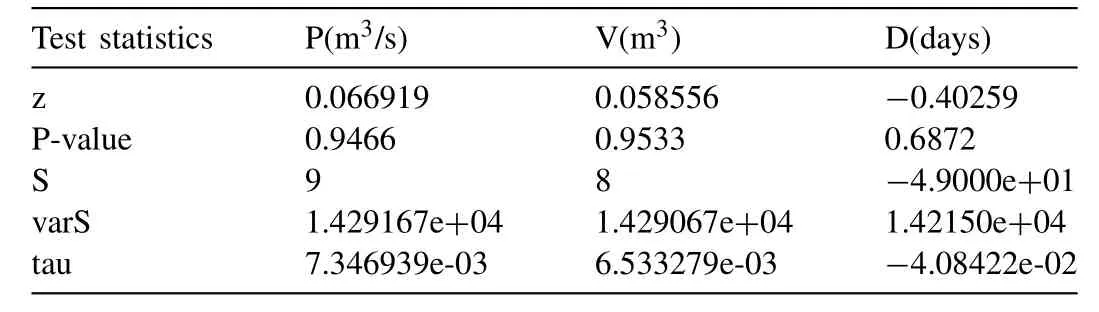
Table6 Mann-Kendall test for testing monotonic trend within flood characteristics.

4.1.2.modellingofunivariatemarginaldistribution

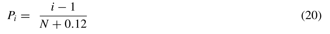
The parametric distribution functions always imposed an assumption that the random samples are coming from the known populations whose PDF are pre-defined.However,no universal rules and studies are imposed to model any hydrologic or flood vectors through any fixed or pre-defined distribution functions,which would follow different distributions and desire to model separately or in other words,the bestfitted marginal distributions are not from the same distribution family.Table1,listed an interactive set of univariate kernel density functions which are employed and tested in this literature,for approximating the marginal probability distribution for individual flood characteristics.The optimal bandwidth of the candidate kernel density functions for three sets of flood characteristics is estimated using Eq.(4),which is based on the Azzalini [3]and Silverman [74]algorithm.Finally,the PDFs of each flood characteristics are derived from Eq.(3).On another side,the CDFs are derived from the empirical procedure which is based on numerical integration procedure because the nonparametric density approximation did not facilitate any closed for of PDF and CDF [40].Fig.3 illustrated the cumulative distribution plot of the kernel function fitted to flood characteristics.Fitness consistency and data reproducing capabilities of each candidate functions fitted with observational samples are examined by comparing theoretical CDFs against empirical non-exceedance probabilities where,the Gringorten plotting position formulae (i.e.,[89]) is employed in the estimation of the empirical probabilities as given below:

where,’i’ is the smallest observations within the data sets of N flood observations when the data are arranged in ascending order.The best-fitted marginal distribution for each flood characteristics is subsequently selected using different analytically based goodness-of-fit test statistics,such as based on error indices statistics like Mean square error (MSE) and Root mean square error (RMSE) (i.e.,[108]),based on the Kullback- Leibler information measures or [100]based information criteria statistics such as the Akaike information criteria (AIC) (i.e.,[82]),Schwartz’s Bayesian information criteria (BIC) (i.e.,[111]) and Hannan-Quinn Information criteria(HQC) (i.e.,[96,83]).The best-fitted univariate distribution model is one which has the minimum value of MSE,RMSE,AIC,BIC and HQC test statistics.Table7 listed the values of the fitness statistics where the bold letter indicated the best fitted marginal distribution for each flood characteristics because they have the lowest value of MSE (i.e.,0.00022 for peak,0.00016 for volume and 0.00048 for duration series),RMSE(i.e.,0.01483 for peak,0.01287 for volume and 0.02208 for duration series),AIC (i.e.,-419.07 for peak,-433.27 for volume and -379.27 for duration series),BIC (i.e.,-417.16 for peak,-431.36 for volume and -377.36 for duration series),and HQC (i.e.,-418.34 for peak,-432.55 for volume and -378.54 for duration series).Therefore,based on the above results,it is concluded that for all the three flood characteristics,i.e.,P,V and D,it seems to follow the Triweight kernel function for describing the marginal distribution.

4.2.Simulation of bivariate parametric copula function

Before initiating the fitting procedure of two-dimensional copulas function,the strength of dependency amongst the triplet flood characteristics are tested analytically using the Pearson’s linear correlation (r),Kendall’s tau (t) and Spearman’s rho (ρ) and their estimated values are listed in Table8.Analytical investigation reveals that the flood peak and volume pair exhibited a strong positive correlation,but the correlation structure between flood peak-duration and flood volume-duration pair are fragile and negatively correlated.The Graphical based dependency measures amongst the flood attribute pairs are also undertaken using the scatter plot and Kendall’s plots (i.e.,[90]),as illustrated in Fig.4 and 5.The Kendall’s plot is analogous to quantile-quantile (Q-Q)plot such that the deviation of random observations from the main diagonal of K-plot is the indication of inter-dependence otherwise could be revealing for independence when the pot tends to be linear (Genest and Boies 2003,Genest and Favre 2007).Therefore,from the Fig.5,it is revealed that based on Kendall’s plot,which indicating strong positive dependency between flood peak-volume pair as the data are much deviated from the main diagonal but the flood peak-volume and volume-duration random pairs,data are much closer to main diagonal thus indicates for negative and weak dependencies between these flood attribute pairs.Similarly,the scatter plot between flood peak-volume of Fig.4,clearly indicates the existence of positive and robust dependency because the increased density of points is located near the diagonal region(i.e.,close to angle 45°) but weak dependency between peakduration and volume-duration.

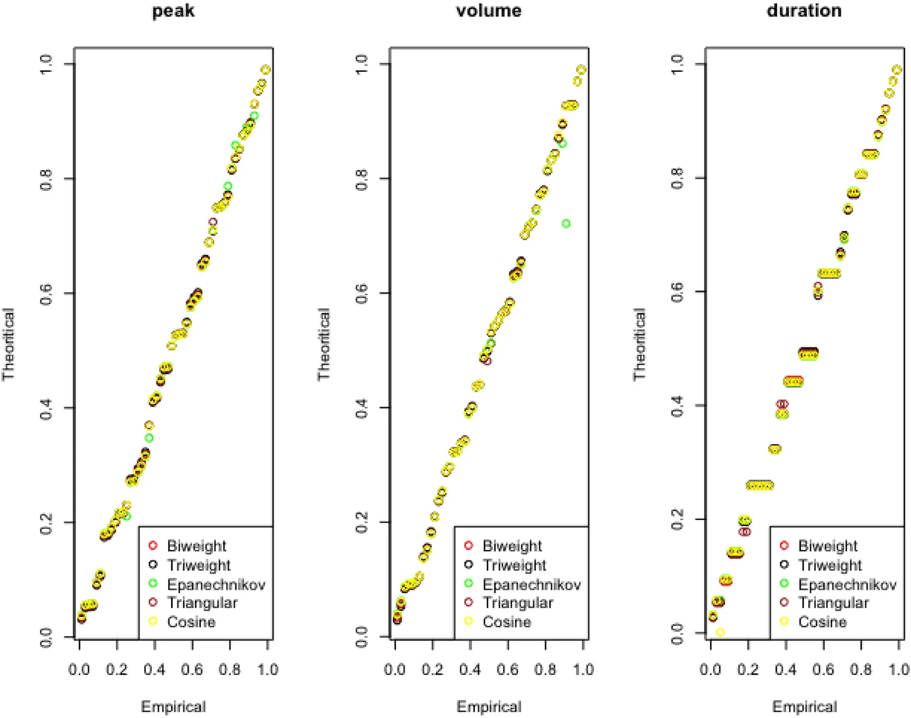
Fig.3.Cumulative distribution plot of the fitted kernel density function.

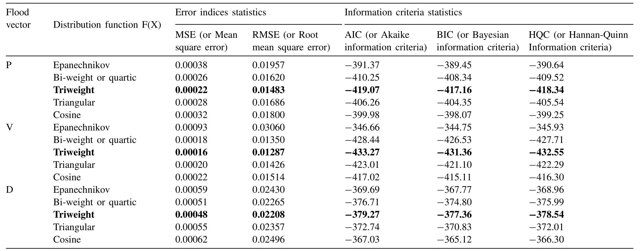
Table7 Comparison of Mean Square Error (MSE),Root Mean Square Error (RMSE),Akaike Information Criteria (AIC),Bayesian Information Criteria (BIC),Hannan-Quinn Information criteria (HQC) values of flood characteristics for different nonparametric univariate probability distributions.

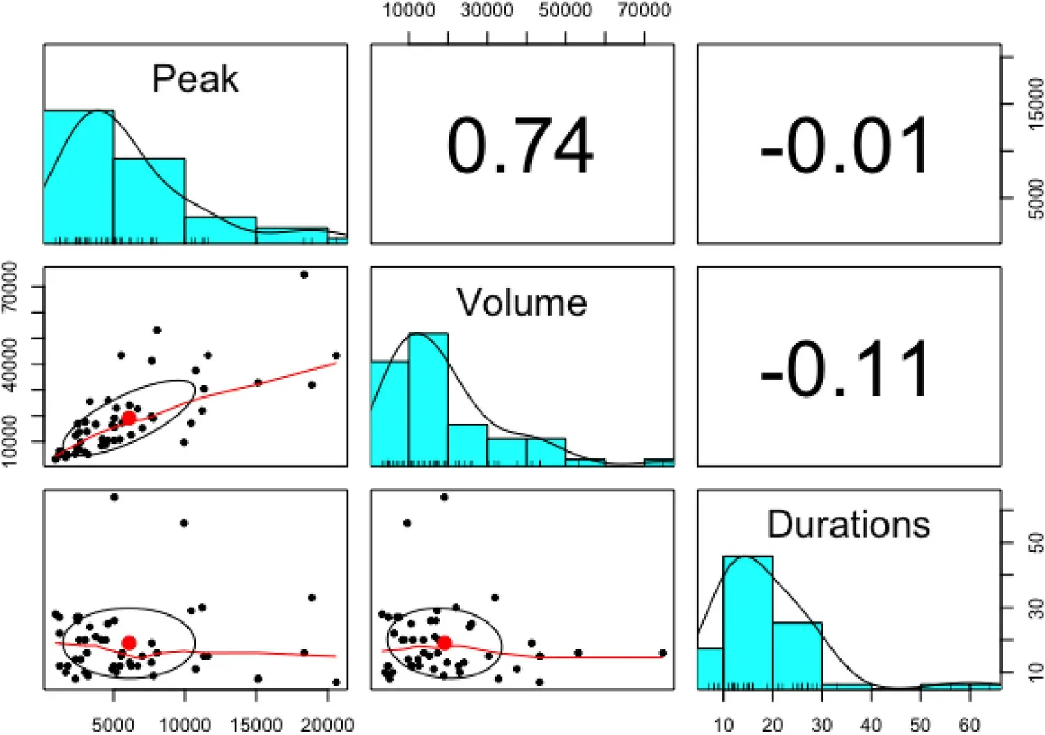
Fig.4.Scatterplot of multidimensional flood characteristics.

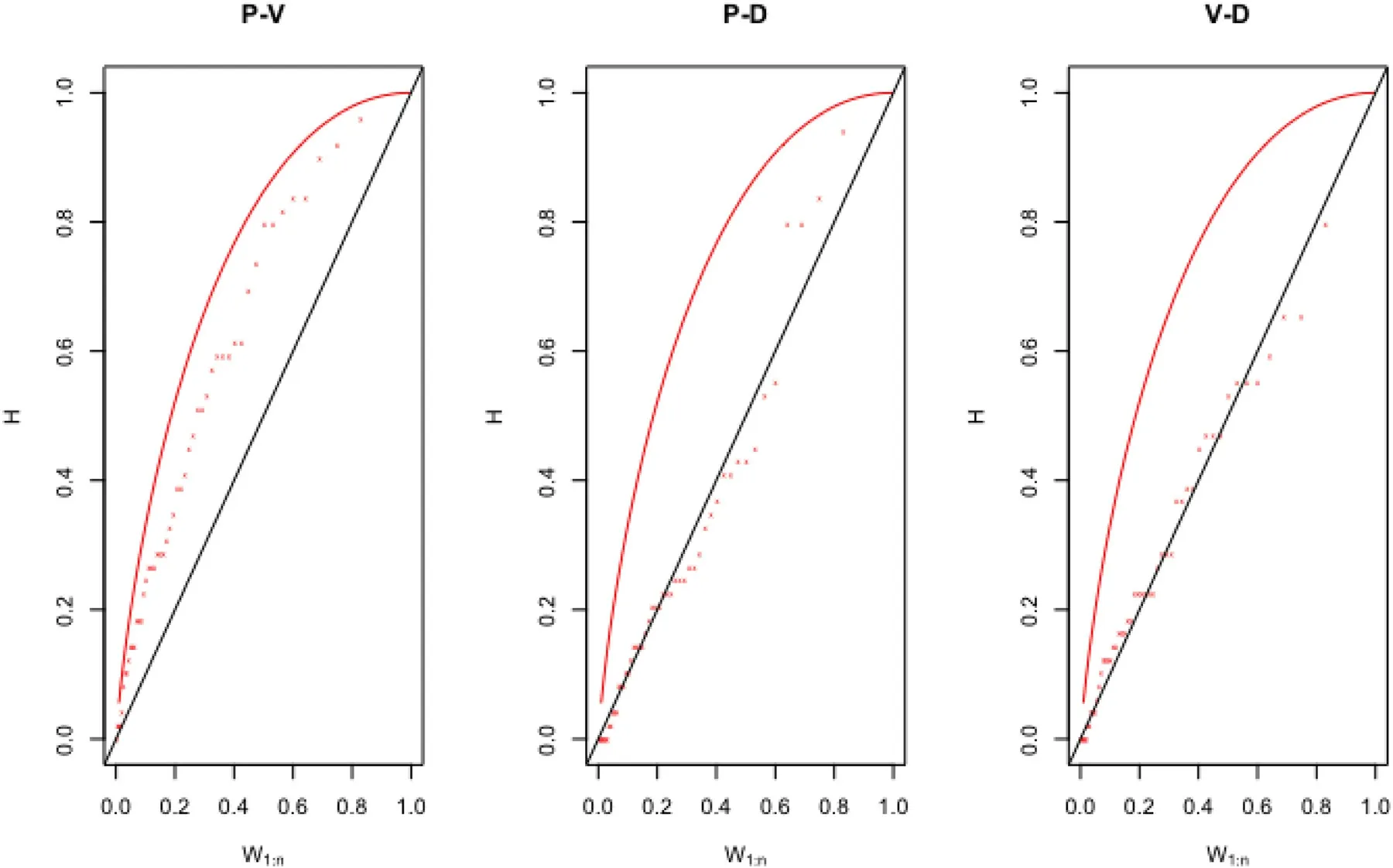
Fig.5.Kendall’s plot (or K-plot) of flood characteristics i.e.,between P-V (shows high and positive correlation structure),P-D (shows negatively correlated random pairs with weak dependency exhibited),V-D (negatively correlated random pairs).

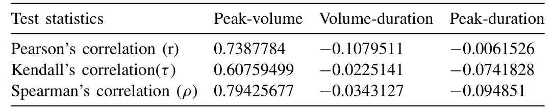
Table8 Dependence measured of analysed flood attribute pairs.

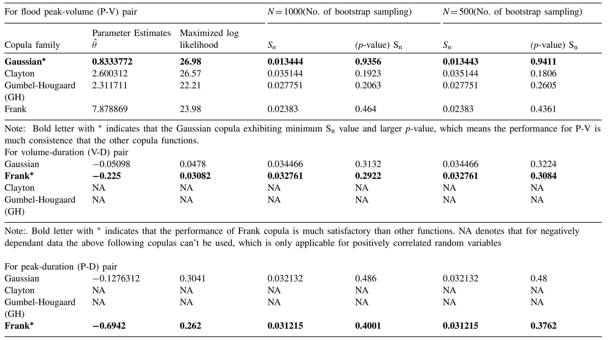
Table9 Copulas dependence parameters based on the Maximum pseudo Likelihood (MPL) estimator and their corresponding goodness-of-fit statistics via parametric bootstrap technique for flood peak-volume,volume-duration,and peak-duration pairs.

In this study,several bivariate copula families such as one elliptical family,i.e.,the Gaussian copula also,the monoparametric version of bi-parametric Archimedean families,i.e.,the Clayton,Gumbel,Frank,are incorporated and then most appropriate copulas are selected for establishing the bivariate joint return periods,i.e.,joint and conditional return periods under the semiparametric copula dependency modelling.The Gumbel-Hougaard and Clayton copula cannot be used for negatively dependant flood characteristics (i.e.,only applicable to model positively correlated random variables).The copulas dependence parameter of the fitted distribution is estimated using maximum pseudo-log-likelihood (or MPL)estimation procedure,using Eq.(11) and their estimated values are listed in Table9.Identification and selection of the best-fitted copulas function for each flood random pairs are performed using the Cramer-von Mises distance statistics with the parametric bootstrap procedure,using Eqs.(13) and 14.The test statistics ‘Sn’ and its associatedp-value have been computed from 1000,and 500 simulated random samples by the mean of the parametric bootstrap procedure and their values are listed in the same Table9.Results revealed that the Gaussian copula exhibited minimum ‘Sn’ statistics and highestp-value for flood peak-volume pair in compare with other peer copula function and thus recognized as the most justifiable for modelling the dependence structure of flood peakvolume pair.Similarly,the Frank copula is identified as most justifiable for capturing the joint structure of both the flood peak-duration and volume-duration pairs,as referred to the same Table9.Finally,the best-fitted copulas selected for each flood attribute pairs are employed to derived joint and conditional return periods.

4.3.Return periods of the flood characteristics and conditional distributions

The hydrologist and water practioner are often interested in the evaluation of the mean inter-arrival period between two design events which usually defined in a year called the return period [112,70,65,33].Mathematically,the univariate return period of the targeted flood characteristics that occurs once in a year are derived from the univariate cumulative distribution function or CDF of the flood variable (say ‘X’),using the best-fitted marginal distribution function,as given below:

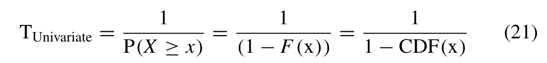
where,TUnivariateis return period in years;F(x) is univariate CDF of the random variable,X,which is derived from best fitted marginal distribution.In the multivariate copula distribution framework,the return period can be estimated in different ways,i.e.,via joint return period and conditional joint return period.The univariate return periods are derived from the best-fitted CDF of flood characteristics,referred to Table10 and illustrated in the Fig.6.

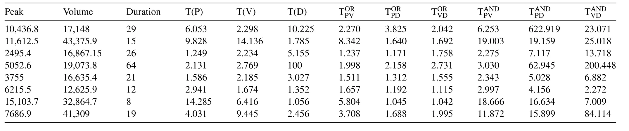
Table10 Univariate and Bivariate joint return periods for flood attribute pairs,peak-volume (P-V),volume-duration (V-D) and peak-duration (P-D).

Fig.6.Univariate return periods derived from the best-fitted cumulative distribution function or CDFs.

4.3.1.Jointreturnperiods

The joint return periods of the bivariate flood characteristics can be derived using the inclusive probability,which is also called ‘OR’ and ‘AND’ cases (i.e.,[65,53]).The joint probability distributions for annual flood analysis can describe the following two situation such that (1) when all targeted bivariate flood variables (say,X≥x,Y≥y,) simultaneously exceed certain threshold during a flood events and their associated return period called the AND joint period and it can be mathematically written in the form,as given below:

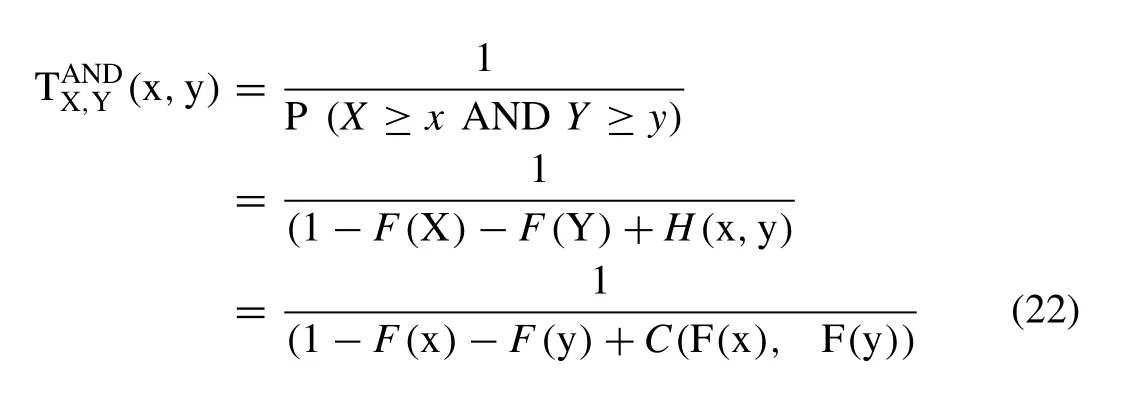
where H(x,y)is the bivariate joint CDF of random variable,X and Y;C(F(x),F(y))is the bivariate copulas CDFs;F(x)=F(y)are the best-fitted univariate marginal distributions.Thus,using the Eq.(22),the joint return periods for‘AND’ case are estimated for different possible combination amongst flood characteristics,i.e.,between peak-volume,volume-duration and peak-duration pairs.Similarly,in the second scenerio,probability either the first or second random variable (say,X≥x,Y≥y) exceed given threshold and thus their associated return period called OR-joint return period that can be mathematically expressed as given below:

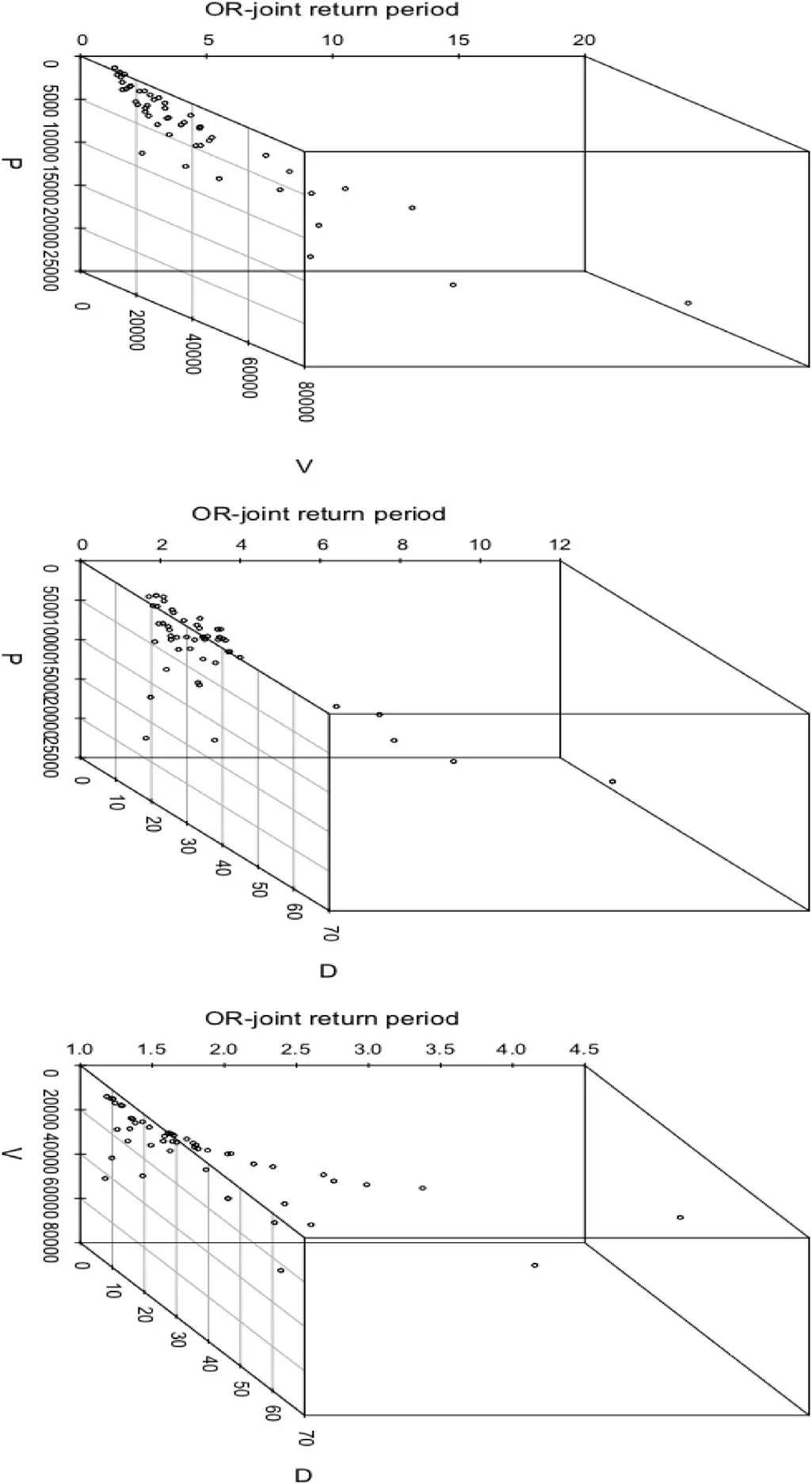
Fig.7.The OR-joint return periods derived from best-fitted bivariate copula fitted flood peak-volume (P-V),volume-duration (V-D) and peak-duration(P-D).

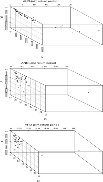
Fig.8.The AND-joint return periods derived from the best-fitted copula fitted flood peak-volume (P-V),volume-duration (V-D) and peak-duration(P-D).

Thus,using the Eq.(23),the OR-joint return periods are estimated for various possible flood combination i.e.,between P-V,V-D and P-D pairs and their values are listed in the Table10.From the Table10 (also,see Figs.7 and 8),it is revealed that the AND-joint return periods produces higher return periods than the OR cases for the same flood combinations i.e.,TORPV＜ TANDPV,TORPD＜TANDPD,TORVD＜ TANDVD.For example,referred to Table10,a flood episode having the flood peak,P=10,463.8 m3s-1,volume,V=17,148 m3,and duration,D=29 days,then the OR-joint return period between P-V is TORPV=2.270 years,between P-D is TORPD=3.825 and between V-D is TORVD=2.042 years.Similarly,the AND-joint return periods for the same events,between P-V,TANDPV=6.253 years,between P-D,TANDPD=622.919 years and between VD,TANDVD=23.071 years (Refer to the same Table10).Similarly,for the flood event describe throughP=5052.6 m3s-1,V=19,073.8 m3andD=64 (days),the OR-joint return period is TORPV=1.998 years (between P-V),TORPD=2.158 years (between P-D) and TORVD=2.731 years but on the other side and the AND-joint return periods for the same flood pairs is TANDPV=3.030 years,TANDPD=62.945,and TANDVD=200.448 years and so on.On the other side,the univariate return periods derived from either flood peak,T(P)or volume series,T(V) is higher than the return periods estimated from OR-joint cases between P-V pairs,i.e.,T(P) ＞TORPVor T(V) ＞ TORPV(referred to Table10).Similarly,the same inequalities are exhibited for the flood volume and duration pairs i.e.,T(V) ＞ TORVDor T(D) ＞ TORVDand also,for the flood characteristics,peak and duration,i.e.,T(P) ＞TORPDor T(D) ＞ TORPD.But on the other side,the ANDjoint cases produces high return periods than those derived from univariate flood characteristics i.e.,TANDPV＞T(P) or TANDPV＞T(V);TANDVD＞T(V) or TANDVD＞T(D);TAND PD＞T(P) or TANDPD＞T(D) (referred to same Table10).Based on the above discussion it is concluded that in the assessments of flood risk,consideration of both the cases of joint return periods i.e.,OR &AND-joint cases could be essential for making a justifiable risk-based decision otherwise accounting based on only either the ‘OR’ or ‘AND’-joint return periods or either based on univariate return periods i.e.,T(P) or T(V)or T(D),would be problematic,and which further might be revealed for underestimations or overestimations of flood risk.

4.3.2.Conditionalreturnperiods

Numerous studies pointed out the necessity of conditional distributional framework and their associated return periods,i.e.,Salvadori and De Michele [70],Shiau et al.,[64],Zhang and Singh [79,80],Reddy and Ganguli [58],Zhang et al.,(2016),Naz et al.,[53].In actual,the conditional return periods relies on the conditional probability between the flood characteristics given that some condition is fulfilled,for example,the conditional return period of flood peak given various percentile value of flood volume or vice-versa.To that end,conditional distributions based on different conditions are estimated first,and then their associated return periods are also derived.Therefore,the conditional return periods of variable,say X given variable,say ‘Y’(Y≤y)(or vice-versa) can be obtained from the conditional probability distribution function is given by:

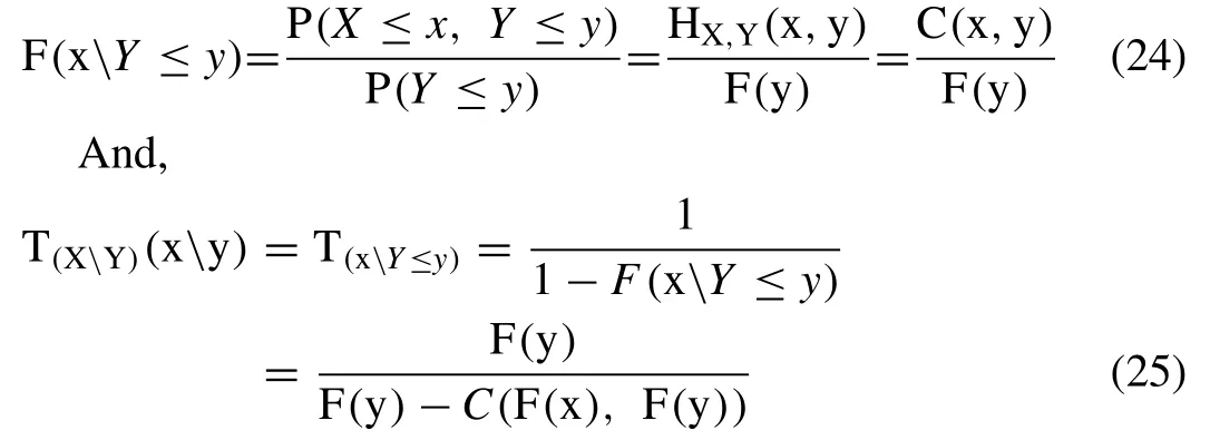
where,C(x,y)is the bivariate copula CDF of random variable X and Y;F(x)=F(y)are the best-fitted univariate marginal distribution functions.Overall,using the Eq.(25) the return periods of one flood variable conditioning to another variable for any possible combination of flood characteristics are estimated and their values for different possible flood combination are listed in the same Table11.For example,a flood event characterized with flood peak flow,P=10,463.8 m3s-1,volume,V=17,148 m3and duration,D=29 (days),using Eq.(25),the joint return period of peak flow conditional to volume is T(p V≤v)=106.9238 years,similarly,the return period of peak flow conditional to durationis T(p D≤d)=5.51532 years and the return period of volume conditional to duration is T(vD≤d)=2.30299 years Similarly,a flood episodes characterized withP=15,103.7 m3s-1,V=32,864.7 m3;D=8 days,the return of ‘P’ conditional to ‘V’ is T(p V≤v)=51.3830844 years,‘P’ conditional to ‘D’ is T(p D≤d)=5.44165 years and ‘V’conditional to ‘D’ is T(vD≤d)=4.08374 years.From the above result and referred to Table11,it is clearly concluded that the conditional return periods between P-V produces higher return value than between P-D and V-D pairs(referred to Table11).Also,the OR-joint return periods between P-V,produces lower return periods than the return periods of flood peak conditioning to volume series,i.e.,Similarly,the OR-joint return periods between P-D &V-D pairs produces relatively lower return periods than the return periods of flood peak conditioning to duration or volume conditioning to duration series,i.e.,

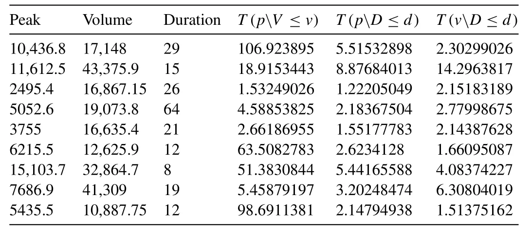
Table11 Conditional return periods for flood attribute pairs,peak-volume (P-V),volume-duration (V-D) and peak-duration (P-D).

5.Research conclusions

The Kelantan River basin is often subject to the most severe monsoonal flooding in Malaysia and perceiving for increasing in term of their frequency and magnitude.The joint distribution analysis,amongst the various intercorrelated flood characteristics,i.e.,flood peak discharge flow,volume and duration always provide a comprehensive understanding and critical hydrological behaviour of the flood episodes in the assessments of hydrologic risk through visualizing the flow exceedance probability or return periods.In this literature,the semiparametric copula-based methodology is incorporated in the bivariate distribution analysis of the flood characteristics and applied as a case study for the Kelantan River basin in Malaysia.In this demonstration,we demonstrated the efficacy of copula-based methodology in the presence of nonparametric based univariate marginal construction.The existing literature mostly focused on the parametric copula modelling approach where the marginal distribution often modelled using parametric distribution functions.However,in actuality,no universal rules and literature are imposed to approximate any hydrologic vectors through any fixed density function,which would follow the different distribution and needs to model.On the other side,the copula function already relaxes the restriction of selecting marginal distributions from the same distribution families.Also,the hydrologic or flood vector mostly exhibited unsymmetrical or non-Gaussian distribution behaviour.In such circumstances,nonparametric kernel density estimations or KDE would be much more stable and less biased smoothing procedure and have better-reproducing capabilities of the random observation than the parametric approach in the approximation of the marginal structure before introducing into copula functions,which relaxing the restrictions of any pre-defined distributions.

The semiparametric copula-based methodology is constructed for the block (annual) Maxima-based flood characteristics for the 50-years (1961-2016) continuously-distributed streamflow characteristics of this river basin.Based on the Pearson,Kendall’s tau and Spearman rho correlation coefficient between the flood characteristics.It is revealed that the flood peak flow-volume pair exhibited positive dependency,but volume-duration and peak-duration pairs are found to be negative and weak correlation.The graphical visual inspection based on the ranked based scatter plot and the K-plot is also illustrated,which are also in support of the analytically based dependency measures.An interactive set of univariate nonparametric kernel density functions are incorporated and tested in for approximating the marginal probability distribution for individual flood characteristics where,the bandwidth of each fitted kernel functions is estimated using optimal bandwidth algorithm (i.e.,[3]and [74]algorithm).Based on the different goodness-of-fit test,i.e.,AIC,BIC,HQC,MSE and RMSE statistics,it is pointing towards the Triweight kernel density function recognized as most justifiable for describing the univariate marginal distribution of flood peak,volume and duration series.Distinguished varieties of bivariate copulas families such as the mono-parametric (or 1-parameter) Archimedean copulas (i.e.,Clayton,Frank,Gumbel) and one Elliptical family copula,i.e.,the Gaussian copula function have been incorporated and tested to model the bivariate joint probability distribution between flood peak-volume,volume-duration and peakduration pairs,where the copulas dependence parameters are estimated using maximum pseudo-likelihood (MPL) estimators.The performance of each fitted bivariate copula function is tested using the Cramer Von-Mises test statistics where the approximation ofp-values for test statistics are obtained using the parametric bootstrapping approach.The test statistics‘Sn’ and their associatedp-values are computed from 1000 to 500 simulated random samples.The best-fitted copulas are used for defining the joint and conditional return periods of the flood characteristics.The analysis revealed that the Gaussian copula is recognized as most logical copula function for establishing the bivariate joint distribution of flood peak-volume pair,which exhibited a minimum value of‘Sn’ test statistics,i.e.,Sn=0.013444 andp-value=0.9356.Similarly,the Frank copula exhibited the minimum value of‘Sn’ test statistics the remaining flood attribute pairs,i.e.,Sn=0.032761 andp-value=0.2922 for flood volume-duration pair and Sn=0.031215 andp-value=0.4001,thus recognized as most parsimonious copula function for establishing joint dependency modelling.Finally,the best-fitted copulas are employed to derive the joint and conditional return periods for various possible combinations of flood characteristics.From the above demonstrations,it is concluded that the AND-joint return period is higher than OR-joint return periods for different flood combinations.

There is much scope for applying the semiparametric copula distribution approaches adopted in this paper to drought or even rainfall episodes in other parts of the world.From the present demonstration,it must be concluded that the semiparametric copula construction could be an effective approach of multivariate distribution modelling of hydrologic consequences because there is no predefined assumption of probability density function during the approximation of the univariate marginal distribution,and which is directly retrieved from the distributed random series with a greater extent of flexibility in their univariate function as compared with parametric density estimators.As the copula function has already facilitated to select the best-fitted marginal not necessarily from the same families of the probability distribution function.Also,in the light of the kernel density function,one can capture the marginal behaviour of random samples more effectively than the parametric distribution approach,along with higher stability and less biased.Besides the above demonstration,it would be more effective if we consider a nonparametric copula joint distribution approach because if the targeted copula function belongs to some specific parametric families,it might be problematic if the underlying assumption is violated.Therefore,in such circumstances,these nonparametric copula distribution framework can ameliorate these modelling issues and can be able to produce significant outcomes without assuming a particular form for the multivariate copula distributions or either univariate marginal distribution.In other words,in the nonparametric model simulation procedure,the univariate marginal distributions are modelled with nonparametric,i.e.,kernel approach and their joint dependence structure are modelled using the nonparametric copula framework,i.e.,the Beta kernel function,where the Beta kernel copula function could be a good choice to estimate the bivariate copula density structure [11,57,94].A study performed by Rauf and Zeephongsekul [57],for rainfall characteristics,already revealed that the nonparametric approach could often give better results than a purely parametric approach and also pointed that such multivariate framework can also be applied and tested to flood or drought episodes in any part of the world.In actuality,no one could deny from the fact that both the nonparametric and semiparametric copula distribution approaches have not been incorporated and exploited to any great extent.In our future research,the nonparametric copula distribution analysis will be a tackle for the same river basin for assessing the flood risk.

Declaration of Competing Interest

None.