Boundary Gap Based Reactive Navigation in Unknown Environments
2021-04-22ZhaoGaoJiahuQinSeniorMemberIEEEShuaiWangStudentMemberIEEEandYaonanWang
Zhao Gao, Jiahu Qin, Senior Member, IEEE, Shuai Wang, Student Member, IEEE, and Yaonan Wang
Abstract—Due to the requirements for mobile robots to search or rescue in unknown environments, reactive navigation which plays an essential role in these applications has attracted increasing interest. However, most existing reactive methods are vulnerable to local minima in the absence of prior knowledge about the environment. This paper aims to address the local minimum problem by employing the proposed boundary gap(BG) based reactive navigation method. Specifically, the narrowest gap extraction algorithm (NGEA) is proposed to eliminate the improper gaps. Meanwhile, we present a new concept called boundary gap which enables the robot to follow the obstacle boundary and then get rid of local minima. Moreover, in order to enhance the smoothness of generated trajectories, we take the robot dynamics into consideration by using the modified dynamic window approach (DWA). Simulation and experimental results show the superiority of our method in avoiding local minima and improving the smoothness.
I. INTRODUCTION
IN recent years, autonomous robot navigation in unforeseen circumstances has received a considerable amount of attention due to the requirements for some special missions,such as exploration and rescue [1]. One of the major challenges is that the robot should reach the goal location without any prior knowledge of the environment. A promising way is to incorporate the sensor information (e.g., laser scanners [2], [3] or cameras [4]) within the control loop,which is the basic idea of reactive collision avoidance methods [5]. By this means, the distribution of obstacles surrounding the robot is detected in real time, so that the robot can achieve collision-free behavior while approaching the goal. However, most reactive methods always suffer from classic problems such as falling into local minima, tendency to oscillate in a narrow passage, and the difficulty of generating the motion towards the obstacle or away from the goal [2].
For tackling the above issues, researchers have made a great deal of effort to improve the existing reactive methods. One of the early works is the artificial potential field (APF) based method proposed in [6]. It assumes that the robot is subjected to attractive and repulsive forces generated by the goal and obstacles respectively. Then, the control command is determined based on the resultant force. However, [7] has shown that this method can easily drive the robot to fall into local minima. One reasonable approach is to build an environment map [8] or a local roadmap [9] online, which is time-consuming to implement. Other efforts including feasible temporary target, virtual obstacle and fuzzy logic are made in[10]–[12]. However, the capability of remedying trap is limited to some specific scenarios since the APF based methods lack further analysis of the environment surrounding the robot.
A representative method to cope with local minimum issue is the Bug algorithm [13], and its numerous variants [14]–[17]have been derived over the years. The key idea of these algorithms is that the robot moves towards the goal until the obstacle is encountered, and then it is drived along the obstacle border till the goal is navigable again, which guarantees global convergence to the goal. In spite of the fact that Bug algorithms possess the capability of tackling local minima, the robot is assumed to be able to follow the boundary of an obstacle with arbitrary shape, and how to achieve the capability has not been considered. Additionally,most methods do not analyze whether the free area is wide enough for the robot to pass since the robot is modeled as a point.
In order to make full use of sensor data for navigation task,the gap based methods have been proposed which analyze the form of high-level descriptions of the environment based on sensor information to determine subsequent actions. The earliest gap based method is nearness diagram (ND) proposed in [2] which takes different control laws according to the predefined configurations of surrounding obstacles. In order to remove abrupt transitions in behaviors, [18] describes the smooth nearness diagram (SND) which adopts a single motion law for all possible situations. Hereafter, the closest gap (CG)presented in [19] highly reduces the number of inappropriate gaps by proposing a new methodology for analyzing gaps.Moreover, the admissible gap (AG) in [20] pays attention to the visibility of the gap. Other variants described in [21], [22],focus on enhancing the smoothness of the trajectories in dense scenarios. Although the widely used gap based methods have shown superior performance, especially in cluttered environments, these methods still have drawbacks while navigating in complex and unknown situations. For instance,some incorrect gaps may be collected due to defects in extracting gaps. Meanwhile, the robot is prone to local minima since almost all of these methods select the closest gap as the target gap. Furthermore, in most work, the dynamics constraints of the robot are ignored, which can lead to collisions.
Rather than methods mentioned before where the appropriate steering direction is calculated, other works focus on choosing control inputs from the velocity space while respecting the vehicle dynamics, such as dynamic window approach (DWA) [23] and its extensions [24]–[27]. The DWA reduces a two-dimensional search space of translational and rotational velocities to the admissible velocities by taking various constraints into account. The velocity pair maximizing the objective function is chosen as the control input to improve the performance of trajectories. Although DWA considers the vehicle dynamics, it blindly guides the robot to approach the goal, which tends to make it fall into local minima. Another popular approach is the velocity obstacles(VO) based method presented in [28]–[31], which ensures the motion safety in dynamic environments. Its basic idea is to determine the set of velocities causing a collision, and select the appropriate velocity outside of the set. The VO based methods show strong obstacle avoidance performance in large-scale dynamic environments, but pay little attention to trap situations.
The motivation of this paper is to address the local minimum problem by utilizing the superior performance of gap based methods in analyzing sensor information. In addition, we are also committed to effectively extracting gaps and enhancing the performance of the generated trajectories.From these points of view, we propose a novel boundary gap(BG) based reactive navigation method in unknown environments. More specifically, the robot detects all traversable gaps by analyzing discontinuities made up of two adjacent scan points, and then the boundary gap is selected among the obtained gap set, which is based on the basic idea that following the obstacle boundary ensures the robot to get rid of traps. Finally, a collision-free motion control is employed to steer the robot through the boundary gap, while respecting the vehicle dynamics. Overall, The main contributions of our work are summarized as follows.
1) The narrowest gap extraction algorithm (NGEA) is proposed which extracts the narrowest gap to evaluate the accessibility reliably.
2) We present the boundary gap which is a new concept for reactive navigation, and design a strategy of identifying the boundary gap that enables the robot to move along the obstacle boundary, which can lessen the possibility of ending in local minima. To the best of our knowledge, it is the first time to employ the gap based method to tackle the local minimum problem.
3) The navigation performance in terms of the trajectory smoothness is improved by applying a modified dynamic window approach (DWA) into our framework.
The remainder of this paper is organized as follows. First,Section II explains the details of BG method. Then, results of the simulation and experiment are shown in Section III.Finally, Section IV concludes our work.
II. BOUNDARY GAP BASED NAVIGATION METHOD
Boundary gap based navigation method for driving a mobile robot in the unknown environment is explained in this section.The framework of the proposed method is shown in Fig.1.First, in each control cycle, all traversable gaps are extracted by analyzing lidar data, which is described in Section II-B.Second, a novel strategy is adopted to select the boundary gap among obtained gaps, which is presented in Section II-C.Third, the desired motion direction along which the robot can travel through the boundary gap is determined in Section II-D.Finally, modified dynamic window approach introduced in Section II-E is applied to control the robot to move safely in the desired direction. Some symbols used in this section have been summarized in Appendix.
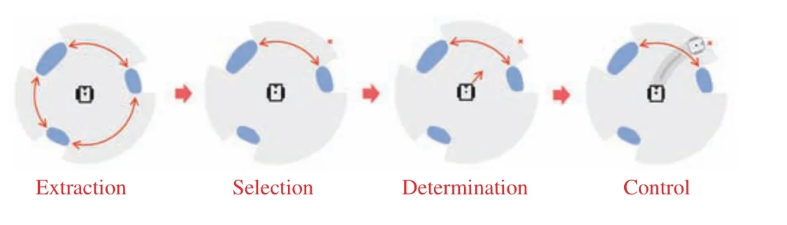
Fig.1. Framework of boundary gap based navigation method.
A. Definitions
1) Mobile Robot: In this paper, we consider a differentialdrive robot (see Fig.2). It is approximated by a circle of radius Rrob. Let R be the robot coordinate frame whose origin is or. The positive x-axis xrcoincides with the robot heading direction. The positive y-axis yris the normal on the left side of xr. Additionally, the goal direction relative to the frame R is denoted by θg.
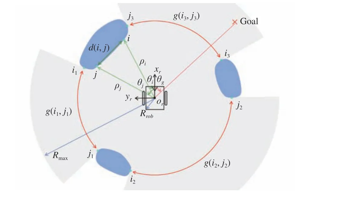
Fig.2. An example of a robot detecting obstacles.
2) Lidar: As shown in Fig.2, the robot equips with a lidar to measure the distance between the robot and obstacles. Let the sensor coordinate frame S coincide with the frame R for simplicity. The detectable area of the lidar is denoted by a circle of radius Rmaxcentered at or. It provides Nsequally angular spaced readings, and each angular interval is denoted by Nθ. Let the first beam whose index is 0 coincide with xraxis, and the index starts to increase from 0 to Ns−1 in a counterclockwise manner. The information of scan point i is denoted by pi=(ρi,θi) in polar coordinate, where ρirepresents the measured distance and θi∈[−π,π) represents the measured angle.
3) Gap: The gap is a obstacle-free opening which indicates a potential path to the occluded area. A gap whose right side and left side indices are i and j respectively is denoted by g(i,j). The gap set consisting of N gaps can be represented as G={g(s1,r,s1,l),g(s2,r,s2,l),...,g(sN,r,sN,l)}, and the side set is denoted by S ={s1,r,s1,l,s2,r,s2,l,...,sN,r,sN,l} . si,rand si,lrepresent the right side and the left side of the i-th gap,respectively. Note that the values of sides si,rand si,lare actually their indices. Similarly, the right side set is denoted by SR={s1,r,s2,r,...,sN,r}, and the left side set is given by SL={s1,l,s2,l,...,sN,l}. For example, three gaps are detected in Fig.2 and form a gap set G={g(i1,j1),g(i2,j2),g(i3,j3)}. Its side set is S ={i1,j1,i2,j2,i3,j3}. The right side set and left side set are SR={i1,i2,i3} and SL={j1,j2,j3}, respectively.
4) Functions: For ease of description, several useful functions are proposed, some of which are introduced in [18].Let S be the unit circle attached to the robot frame R and the positive rotation direction is counterclockwise.
Given angles α,β ∈S, the angular distance dist(α,β) is denoted by

where distc(α,β)=((α−β)mod 2π) and distcc(α,β)=((β−α)mod2π) are angular distances from α to β in clockwise and counterclockwise directions, respectively. In addition, the direction depending on α and β is defined as

where c and cc represent the clockwise and counterclockwise directions respectively. Note that the first parameter in above functions would be omitted if it equals zero.
The distance function d(i,j) is used to calculate the Euclidean distance between two scan points i and j. It is given by
where (ρi,θi) and (ρj,θj) are the polar coordinates of scan points i and j, respectively.
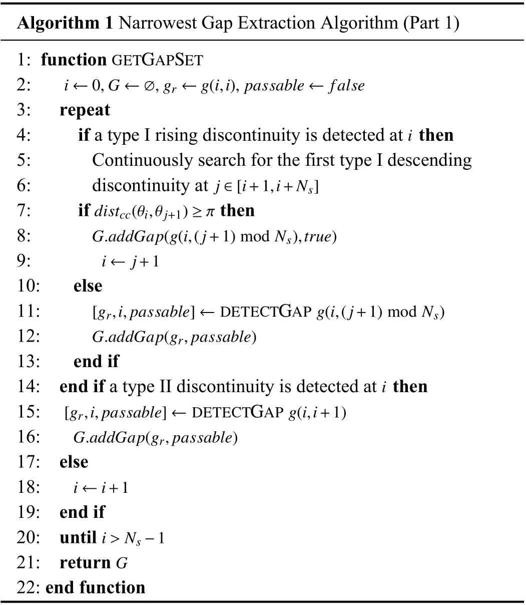
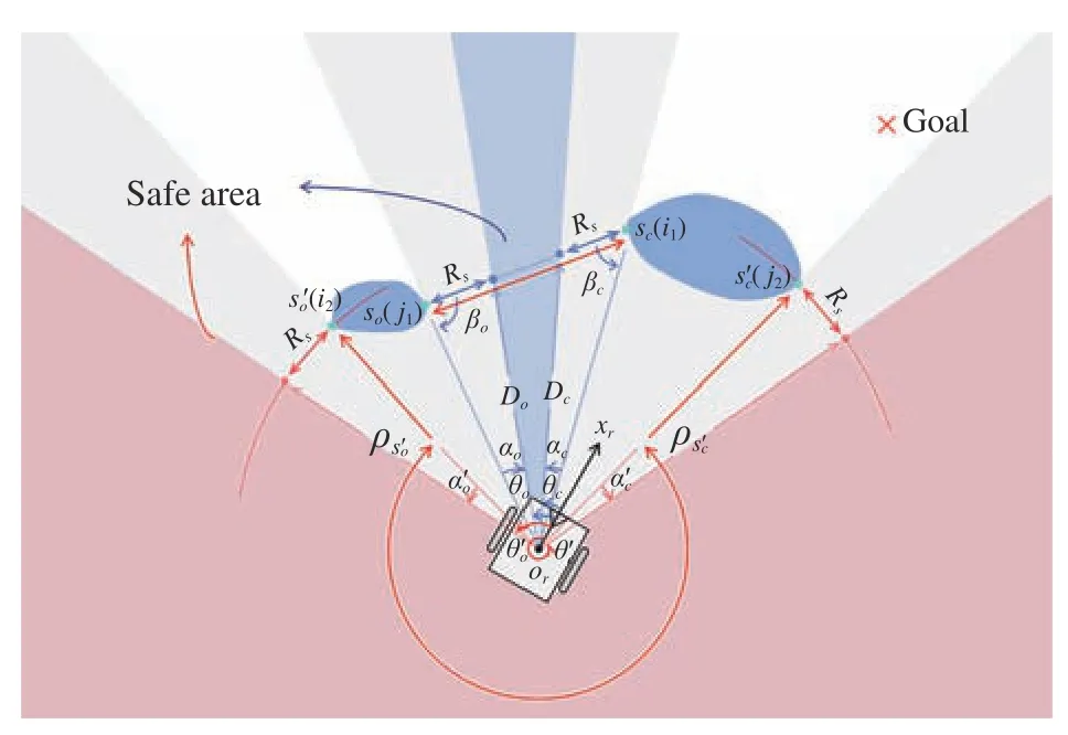
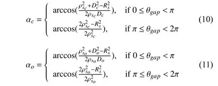
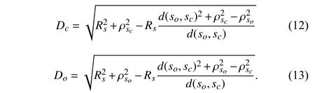
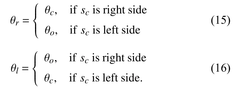
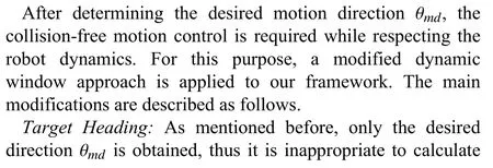
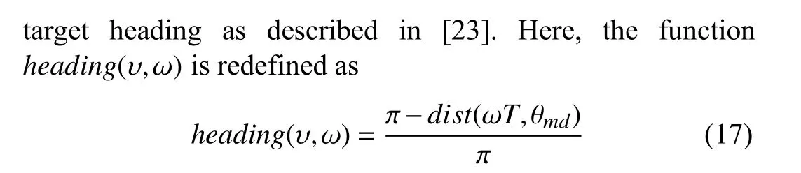
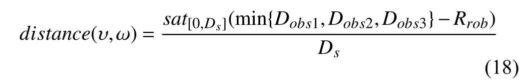
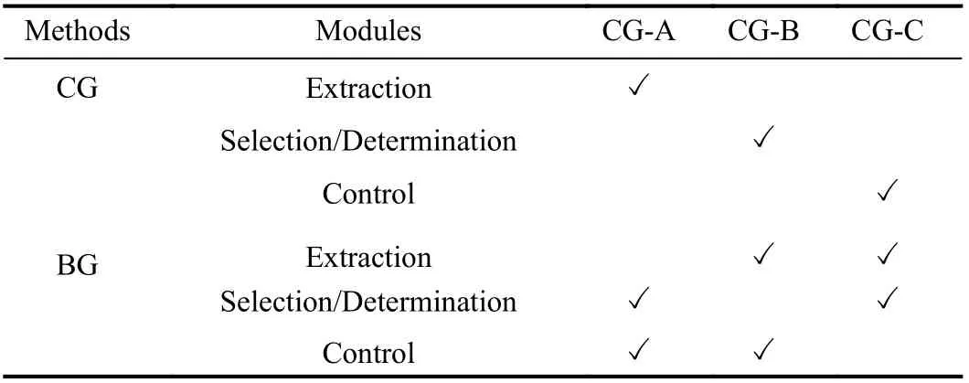
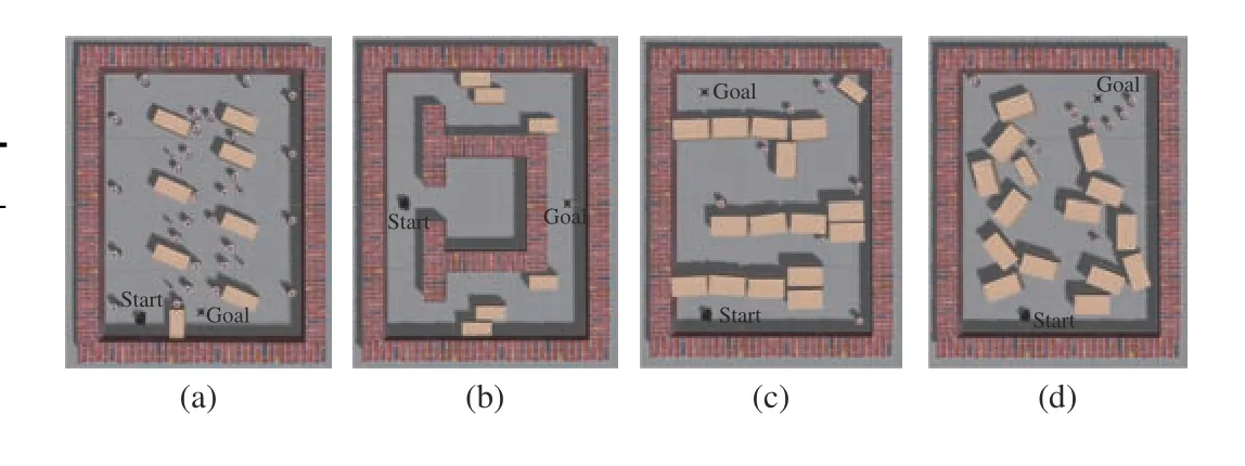
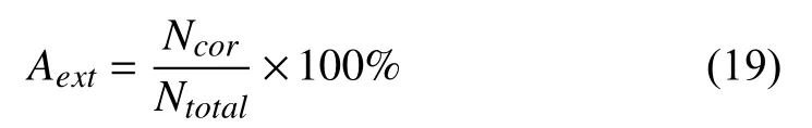
Given a In order to determine all accessible regions, extracting gaps is performed based on the structure of obstacles around the robot. First of all, two types of discontinuities defined in [19]are introduced. Given contiguous scan points i and j (j>i),they are defined as follows. Type I Discontinuity: It occurs if one of two distance measurements of scans i and j returns Rmax, i.e., Type II Discontinuity: It occurs if the distance between scans i and j exceeds the predefined safe threshold, i.e., where Rsrepresents the safe radius which is slightly larger than the robot radius Rrob. A rising discontinuity occurs at i if ρj>ρi, and a descending discontinuity occurs at j otherwise. By the way,the priority of type I discontinuity is higher in our method,which is different from that described in [19]. Algorithm 1 Narrowest Gap Extraction Algorithm (Part 1)1: function GETGAPSET i ←0,G ←∅,gr ←g(i,i),passable ←false 2: 3: repeat 4: if a type I rising discontinuity is detected at then 5: Continuously search for the first type I descending j ∈[i+1,i+Ns]i 6: discontinuity at distcc(θi,θ j+1)≥π 7: if then G.addGap(g(i,(j+1)mod Ns),true)8: 9: 10: else[gr,i,passable]←g(i,(j+1)mod Ns)i ←j+1 11: DETECTGAP G.addGap(gr,passable)12: 13: end if 14: end if a type II discontinuity is detected at then[gr,i,passable]←g(i,i+1)i 15: DETECTGAP G.addGap(gr,passable)16: 17: else i ←i+1 18: 19: end if i>Ns −1 20: until 21: return 22: end function G Fig.5. Safe areas in two cases. Blue and red safe areas correspond to cases 0 ≤θgap<π and π ≤θgap<2π, respectively. θc and are right border d irections. θo andare left border directions. where αcand αoare safe angular distances to the closest side and other side, respectively. They are given by where θgaprepresents the angular width of the gap, and the distances Dcand Doare given by Then, the motion direction θmdis defined as where right border direction θrand left border direction θlare g iven by where T is total time horizon. Its value is maximal if the robot heading at predicted position coincides with the direction θmd. Clearance: The clearance function distance(υ,ω) returns the minimum distance between the predicted trajectory and obstacle points. It is redefined as where Dsis a tuning parameter that indicates the safe distance the robot keeps from obstacles, Dobs1indicates the minimum distance from the predicted position to the obstacle, Dobs2and Dobs3represent the shortest distances between the predicted trajectory and obstacles on its sides. These three parameters are intuitive in Fig.6. Fig.6. Clearance analysis. The predicted trajectory is represented by a dark gray circular arc with a circle center ot lying on the positive y-axis yr. In this section, we evaluate the effectiveness of the BG method by implementing experiments. First, we generate different methods for comparison, and four well-designed scenarios are used for simulation. Second, some quantitative metrics are defined to assess the performance of the algorithm.Third, the simulation experiment is carried out and the results are analyzed. Finally, the implementation in the real world scenario is also organized to demonstrate the feasibility of the proposed BG method. We consider the classic CG method as a contrast, which also focuses on effectively extracting the narrow gap. In addition, in order to evaluate the performance of each module of our algorithm, we combine different modules of BG and CG methods to generate new methods for comparison, i.e.,CG-A, CG-B and CG-C methods (see Table I for details). We design four representative scenarios (4×3 m) created in Gazebo (see Fig.7 ), a popular 3-dimensional simulation software. As shown in Fig.7(a), a number of cans and boxesare distributed in Scenario I, which creates many irregular gaps. Thus it is mainly used to evaluate the performance of gap extraction algorithm. Figs. 7(b) and 7(c) give a large Ushaped structure and a narrow S-shaped curved passage,respectively, which are common trap environments. In Fig.7(d), a cluttered environment without traps is used to test the smoothness of the algorithm. TABLE I MODULE COMBINATION OF NEw METHODS Fig.7. Simulation scenarios: (a) Scenario I; (b) Scenario II; (c) Scenario III;(d) Scenario IV. TABLE II OVERALL PERFORMANCE IN FOUR SIMULATION SCENARIOS. BEST SCORES ARE HIGHLIGHTED IN BOLD To evaluate the performance of each method quantitatively,the following metrics are employed. Total Time(Ttotal): The time taken to reach the goal. Trajectory Length(Ltraj): The total path length to reach the goal. Extraction Time(Text): The average time taken to extract gaps. Extraction Accuracy(Aext): The accuracy of gap extraction.It is defined as where Ncorrepresents the number of control cycles in which the gap leading to the goal is selected, and Ntotalrepresents the total number of control cycles. Curvature Change(Ccurv): It reflects the oscillation of the trajectory. It is defined as [34] where k(t) is the curvature of the trajectory at time t. Linear Jerk(Jline): It is used to measure the smoothness of linear velocity. It is defined as [22] where v(t) is the linear velocity at time t. Rotational Jerk(Jrot): It is used to measure the smoothness of angular velocity. It is defined as [22] where w(t) is the angular velocity at time t. For the sake of visualization, simulation is executed in MATLAB on a computer with Intel i3-8100 CPU and 8 GB of memory. During the simulation, we use a circular differentialdrive simulated robot with radius 0.105 m, which is equipped with a full field of view lidar. Its maximum linear and angular velocities are set to 0.22 m/s and 2.84 rad/s, respectively.Since reducing the maximum detection range can increase the possibility of falling into local minima [35], we limit its maximum detection range to 1.0 m. Fig.8. Simulation results. (a)–(c) Results in Scenario I using (a) CG, (b) CG-A and (c) BG; (d)–(f) Results in Scenario II using (d) CG, (e) CG-B and (f) BG;(g)–(i) Results in Scenario III using (g) CG, (h) CG-B and (i) BG; (j)–(l) Results in Scenario IV using (j) CG, (k) CG-C and (l) BG; Note that the dotted line indicates the gap and the blue dotted line indicates the target gap. Fig.9. Experimental results. (a) Experimental scenario; (b)–(m) Snapshots of the navigation process; (n) Desired linear velocity and actual linear velocity curves; (o) Desired angular velocity and actual angular velocity curves. Table II shows the quantitative results of the different methods in four scenarios. The resulting trajectories can be seen in Fig.8. In Scenario I, the CG-A method has obvious oscillation due to selecting the improper gap (see Fig.8(b)).However, the BG method effectively improves this issue and avoids unnecessary movements (see Fig.8(c)). Meanwhile,the extraction time of our method is shorter than that of the CG-A method, which suggests that our extraction algorithm has better real-time performance. In Scenarios II and III, the major challenge is to escape the trap. As shown in Figs. 8(d),8(e), 8(g), and 8(h), since the unreasonable strategy makes the desired motion direction exchange repeatedly, the robot oscillates and eventually stagnates in place. In fact, the reason why the robot employing the CG method in Scenario I failed to the goal is the same. Instead, the goal has been reached successfully using the BG method as shown in Figs. 8(f) and 8(i).In Scenario IV, all three methods lead the robot to reach the goal (see Fig.8(j)–8(l)). However, the performances are not the same. As shown in Table II, our BG method delivers significantly better results, e.g., smoothness, due to the consideration for the robot dynamics. We have carried out our reactive obstacle method in the physical reality with the TurtleBot3 Burger which is a programmable differential mobile robot. It has a rectangular shape (0.138× 0.178 m) and is equipped with an on-board computer (Raspberry Pi 3). Its maximum linear and angular velocities are 0.22 m and 2.84 rad/s respectively. The LDS-01,a 2-dimensional laser scanner capable of sensing 360°, is mounted on the Burger. It has a resolution of 1° and maximum distance range of 3.5 m which is also limited to 1.0 m. During the experiment, the robot operating system (ROS) is used for inter-process communication. The position of Burger is estimated by its odometry. The control frequency is set to 20 Hz.Note that we have not provided the occupancy map to the robot so as to simulate navigation in the unknown environment. As shown in Fig.9(a), a relatively narrow curved passage is created to verify the practicality of our algorithm. In this scenario, the robot is vulnerable to local minima since it is required to behave far from the goal. The snapshots of the navigation process are shown in Figs. 9(b)–9(m). It is obvious that the Burger has succeeded to travel through the passage and reached the goal location. The desired linear velocity and actual linear velocity curves are depicted in Fig.9(n), and the desired angular velocity and actual angular velocity curves are drawn in Fig.9(o). We have presented the BG method, a reactive obstacle avoidance approach in unknown environments. First, the narrowest gap extraction algorithm is proposed to eliminate useless gaps and reduce unnecessary movements. Second, by identifying the boundary gap, the robot can follow the obstacle border and get rid of local minima. Moreover, we apply the modified DWA into our framework, which improves the performance of the trajectories in terms of smoothness. Finally, simulation and experimental results show the superiority of our method. Our BG method is suitable for static environments.However, there are dynamic obstacles in most real scenes.Therefore, we aim to extend the BG method to dynamic scenarios in our future work. APPENDIX A. Notations There are many symbols in this paper. In order to improve the readability, the main notations are summarized as follows.
B. Gap Extraction


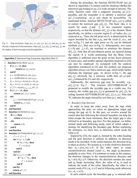


E. Modified Dynamic Window Approach

III. EXPERIMENTS AND RESULTS
A. Experimental Setup

B. Quantitative Metrics


C. Simulation Results

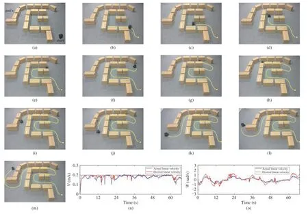
D. Experimental Results
IV. CONCLUSIONS
杂志排行
IEEE/CAA Journal of Automatica Sinica的其它文章
- Physical Safety and Cyber Security Analysis of Multi-Agent Systems:A Survey of Recent Advances
- Joint Algorithm of Message Fragmentation and No-Wait Scheduling for Time-Sensitive Networks
- Multiagent Reinforcement Learning:Rollout and Policy Iteration
- A Survey on Smart Agriculture: Development Modes, Technologies, and Security and Privacy Challenges
- A Survey of Evolutionary Algorithms for Multi-Objective Optimization Problems With Irregular Pareto Fronts
- Dependent Randomization in Parallel Binary Decision Fusion