A Risk-Averse Remaining Useful Life Estimation for Predictive Maintenance

Chuang Chen, Ningyun Lu, Member, IEEE, Bin Jiang, Fellow, IEEE, and Cunsong Wang, Student Member, IEEE

Abstract—Remaining useful life (RUL) prediction is an advanced technique for system maintenance scheduling. Most of existing RUL prediction methods are only interested in the precision of RUL estimation; the adverse impact of overestimated RUL on maintenance scheduling is not of concern. In this work, an RUL estimation method with risk-averse adaptation is developed which can reduce the over-estimation rate while maintaining a reasonable under-estimation level. The proposed method includes a module of degradation feature selection to obtain crucial features which reflect system degradation trends.Then, the latent structure between the degradation features and the RUL labels is modeled by a support vector regression (SVR)model and a long short-term memory (LSTM) network,respectively. To enhance the prediction robustness and increase its marginal utility, the SVR model and the LSTM model are integrated to generate a hybrid model via three connection parameters. By designing a cost function with penalty mechanism, the three parameters are determined using a modified grey wolf optimization algorithm. In addition, a cost metric is proposed to measure the benefit of such a risk-averse predictive maintenance method. Verification is done using an aero-engine data set from NASA. The results show the feasibility and effectiveness of the proposed RUL estimation method and the predictive maintenance strategy.

I. INTRODUCTION

IMPROVING operation quality and reducing operation costs are two major concerns in many enterprises [1]–[3].Unexpected downtimes often mean unbearably high costs.Orienting at Industry 4.0 or made in China 2025, maintenance technology is more attracted to predictability [4]. Based on online condition monitoring information, predictive maintenance (PdM) can output some indicators to show the levels of system health states or the estimation of their remaining useful life (RUL) [5]. These indicators can assist maintenance decision-making, such as to obtain the optimal maintenance time and the ordering time of spare parts. There is an increasingly common view that PdM outperforms traditional maintenance strategies such as time-based maintenance and corrective maintenance. It has attracted considerable attentions in recent years [6]–[10].

RUL estimation is the most important step in a PdM strategy. With the estimated RUL, one can schedule maintenance activities confidently for a degrading system[11]–[13]. There are many studies attempting to improve the precision of RUL estimation. However, few of them considered it from a maintenance perspective. Maintenance scheduling is the ultimate goal of RUL prognostics. In general, an under-estimated RUL is better than an overestimated one under the same or close prediction error,because with over-estimated RUL, the risk of unexpected shutdowns will surge and may sometimes cause disastrous consequences. Therefore, it is necessary and significant to properly correct the misleading RUL estimation and then reduce possible wrong decisions of maintenance scheduling.

To do so, a risk-averse RUL estimation method is proposed for predictive maintenance. Firstly, features that can reflect system degradation trend are selected. Then, the latent structure between degradation features and the RUL labels is modeled by a support vector regression (SVR) algorithm and a long short-term memory (LSTM) network separately, since SVR and LSTM are currently two well recognized prognostics tools. To enhance the robustness of prognostics and increase their marginal utility, the SVR model and the LSTM model are combined via three connection parameters to generate a new hybrid model. The risk-averse adaptation is realized by optimizing the three connection parameters to minimize a cost function online. From the perspective of maintenance scheduling, a cost metric is also developed for measuring the benefit provided by risk-averse prognostics.

The remainder of this paper is organized as follows. Section II reviews the related work. Section III presents a risk-averse RUL estimation method for predictive maintenance. The major steps include selection of degradation features,prognostic model training, risk-averse adaptation, and online prognostics. Verification is conducted using the NASA data set of aero-engines in Section IV. Section V draws the conclusions and discusses the possible future work.

II. RELATED WORK

This section presents the state-of-art of RUL prognostics in recent years. From the perspective of prognostic procedures,these existing RUL prognostics studies can be roughly divided into three branches: degradation state based, regression based,and pattern matching based prognostic methods [14].

For degradation state based methods, RUL is usually estimated in two steps: estimating system health state and then inferring the RUL using a failure threshold. For instance, a fuzzy c-means algorithm was employed to partition the run-tofailure condition monitoring data, and the final RUL was estimated by a multivariate health estimation model and a multivariate degradation prediction model [15]. In [16], the run-to-failure data were divided into four states using several belief functions, and RUL was estimated as the transition duration from the degraded state to the failure state. In [17],RUL was estimated by projection with the combination of degradation modeling and a particle filter algorithm, where the parameters of probability distribution at the last step of online updating were regarded as the final RUL distribution.

The regression based methods are devoted to predicting the evolution behavior of a degradation indicator so that the estimation of RUL can be obtained when the degradation indicator reaches an end-of-life (EOL) criterion. In this branch, support vector regression (SVR) is the mainstream technology. For example, in [18], a particle swarm optimization algorithm was employed to optimize the configuration parameters of SVR; the estimated RUL was obtained by the SVR based one-step time series prediction[19]. In [20], a particle filter and an SVR were combined to estimate the capacity degradation of a lithium-ion battery, and the RUL was defined by the probability distribution parameters.

The above two branches of prognostic methods are strongly dependent on the setting of such failure threshold, which is a challenging issue in practice. The pattern matching based method raises attentions alternatively. They aim to identify the right trend along with its EOL value from the sample datasets.In [21], the degradation was represented as one-dimensional health indicator trajectory using linear regression, and the RUL of the current sample was obtained by comprehensive analysis of similar trajectories. Similar ideas can be found in[22]–[24]. However, the pattern matching method relies on the quality of the sample’s datasets. In the absence of matched patterns, the estimated result is quite wayward.

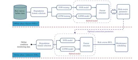
Fig.1. Framework of the proposed PdM strategy.

Recently, two new RUL prognostics methods, which require no estimation of health states or setting of failure threshold,have been published [14], [25]. They attempt to build the direct mapping relationship between degradation features and RUL using data-driven techniques. In [14], SVR was used to build such a direct relationship. In [25], long short-term memory (LSTM) networks were employed. The two models have shown their advantages in higher prognostics precision.

Generally speaking, for a single prediction model,prediction precision shows a trend of diminishing marginal utility [26]. One possible solution is to develop a hybrid model which can maintain the positive parts of each modeling method and prevent the diminishing marginal utility problem of a simple prediction model. For this purpose, a hybrid model that combines the SVR and LSTM models is considered in this paper. Further, on the basis of [14] and [25], the riskaverse adaptation is investigated to contribute to predictive maintenance, which is the main contribution of this paper.

III. METHODOLOGY

A. Key Idea

The scheme of the proposed risk-averse RUL estimation based predictive maintenance strategy is shown in Fig.1. It contains two phases: offline training and online application.

In the offline phase, the raw run-to-failure data (with known EOLs) are first transformed into a set of features using the degradation feature selection module. The features should reflect the degradation trend of the system. Next, the SVR and LSTM models are separately trained for learning the relationship between the features and the RULs. Also, the two models are fused by several connection parameters, and the parameters are determined using an evolutionary algorithm.

In the online phase, the online condition monitoring data(with unknown EOL) are collected and appended to get a section of trajectories, and then processed in the same manner as that in the offline phase to extract degradation features.Right after, the features are fed into the well-trained SVR and LSTM models, and the two models output the estimated RULs independently. The ultimate RUL estimation is obtained by the risk-averse hybrid model for maintenance decisionmaking.

B. Extracting Degradation Features

The process of degradation feature selection can be illustrated in Fig.2. Usually, system degradation is a slow and monotonic process, which means that the degradation features should exhibit certain tendencies [27]. Moving average is a simple but effective skill for tendency extraction. Given a time series {s1,s2,...,sl}, using moving average, the degradation trend (namely the degradation features discussed below) can be obtained, i.e.,

where sidenotes the monitored indicator of system at moment i, and n is the moving window size.

Fig.2. Process of degradation feature selection.

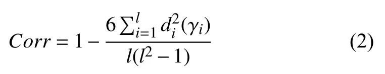
Irrelevant or redundant features affect the performance of learning algorithms. Therefore, it is necessary to eliminate such features and only maintain contributory ones. Correlation and consistency indicators [15] can be employed for such purposes.

The correlation indicator reflects the linear correlation between a feature and the length of an observed sequence,which is formulized as

The consistency indicator reflects the consistent tendency of a feature in all samples, which can be calculated by

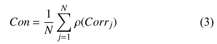
Thus, the rule for extracting the degradation features is to choose the features that satisfy the conditions, |Corr|≥ϑ and Con=0 or 1. Here, ϑ is the correlation threshold and is generally set between 0.5 and 1.

C. Modeling Features-RUL Relationship

This step is to develop a model that can accurately describe the relationship between the degradation features and the corresponding RUL, i.e.,

To the best of our knowledge, SVR and LSTM models are currently two well recognized prognostics models. SVR model was developed from support vector machine (SVM).With an error range, the predicted value falling within the error range is regarded as the correct prediction [28]. SVR is effective in establishing nonlinear mapping relationships because its learning algorithm comes from a convex optimization problem. However, it cannot handle dependencies amongst multiple time series, so it lacks the overall perception ability. LSTM model is a special type of neural network which can handle dependency between successive steps. The mapping relationship is realized by the cooperation of three gates (input gate, forget gate and output gate) [29], [30]. Nevertheless, the LSTM model structure is difficult to optimize, and as a result, its performance is difficult to improve.

As stated before, a hybrid model can maintain the positive aspects of each modeling method and prevent the diminishing marginal utility problem of simple prediction models. Thus, a hybrid model that combines the SVR and LSTM models is developed via three connection parameters ( w1, w2, b), as illustrated in Fig.3. It is noted that to be exact, the ε-SVR and vanilla LSTM models are chosen according to [14] and [25].The fusion structure enables information exchange between the two models. Through such information exchange, a better RUL estimation can be achieved.

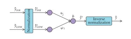
Fig.3. Fusion structure of SVR and LSTM models.

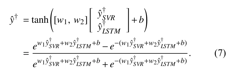
It should be noted that, the activation function of (7) is adopted to handle the nonlinearity of the fusion structure. The fusion structure can be a simple linear expression. However,linear expressions often do not perform well compared with the above nonlinear form. Observed from (7), the range of hyperbolic tangent activation function is between −1 and 1,and this also explains the purpose of normalization using (5)and (6).

Lastly, the RUL estimation is obtained after an inverse normalization, i.e.,

Now, the remaining problem is to determine the three parameters ( w1, w2and b) to meet the design requirement of risk-averse adaptation.

D. Risk-Averse Adaptation

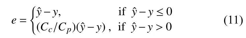
It is a common view that underestimated RUL is relatively better than the overestimated one under the same or close prediction error. Accordingly, the hybrid model should consider the objective of reducing the overestimation rate while maintaining a reasonable underestimation level. In this context, the error function below is given to incline more to the underestimated RUL, i.e.,

Thereupon, the minimization error function (cost function)is defined as

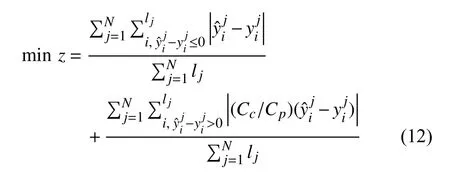
where ljis the RUL sequence length of the j-th sample. With this penalty mechanism, the cost function forces the prognostics to shift from overestimation to underestimation.The values of w1, w2, and b are selected by minimizing the function (12).

Considering the complexity of (12), it is difficult to get a closed-form solution. From a usability standpoint, one can obtain a group of feasible sub-optimal solutions rather than a closed-form optimal solution by using evolution algorithms[31]. In this paper, the grey wolf optimization (GWO)algorithm is selected to estimate the values of w1, w2, and b.

GWO algorithm is an emerging technique in the field of evolutionary algorithms. It is inspired by the intelligent activities of grey wolf population hunting and has been proved to be superior to traditional algorithms, such as genetic algorithm (GA), particle swarm optimization (PSO) algorithm,and differential evolution (DE) algorithm [32]. Unfortunately,the GWO algorithm generates an initial population in a random manner. Although the initial population has a certain population diversity, the population level may not be good,affecting the convergence speed and precision of the algorithm. After randomly generating the initial population,embedding a selection operator will help improve the optimization performance of the GWO algorithm [33]. In addition, the GWO algorithm must balance the global searching and the local searching. Without an effective balance mechanism, the algorithm may fall into local optimum. To overcome this problem, one can modify the convergence factor. More specifically, the linear convergence factor is replaced by a nonlinear convergence factor. The nonlinear convergence factor will drive the algorithm to search globally in the early stage, and turn to local searching later. This improved algorithm is named as GWO-II algorithm in this paper.

Fig.4 shows the implementation process of the GWO-II algorithm. Based on the GWO-II algorithm, the three parameters ( w1, w2, b) can be solved by the following steps.

Step 1: Initialize the parameters, including the population size S, the maximum number of iterations T, and each individual position Qk=(w1,w2,b) with k=1,2,...,S.

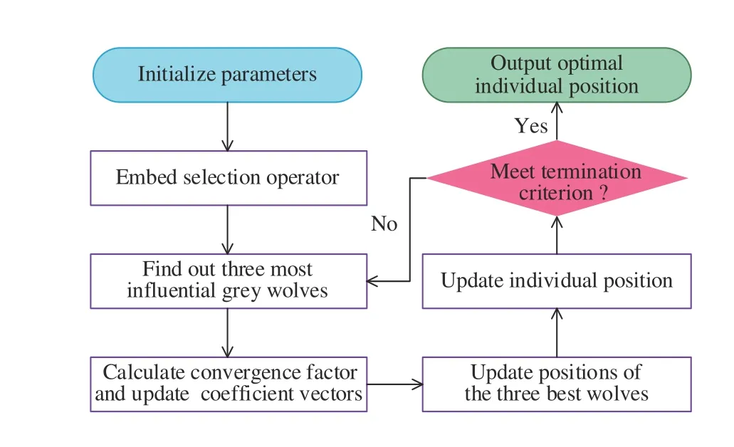
Fig.4. Implementation process of GWO-II algorithm.

Step 2: Embed a selection operator. The fitness values of all individuals in the population are first calculated according to(12). Subsequently, these fitness values are arranged in ascending order. All individuals are divided into the front,middle, or back segment. Individuals in the front are better solutions. Finally, each segment is randomly selected according to the proportion of 1.0, 0.8, and 0.6. For the individuals who lost 20% in the middle segment and 40% in the back segment, the individuals in the front segment are supplemented to form a new population with the same population size.

Step 3: Find out the three most influential grey wolves in the new population. They are noted as α, β, and δ in turn. The three wolves will lead the population to surround, hunt and attack the prey (target solution).

Step 4: Calculate the convergence factor and update the coefficient vectors. The proposed convergence factor ϖ is reduced from 2 to 0 in a nonlinear way of (13). After that, the coefficient vectors A and C can be updated by (14) and (15).

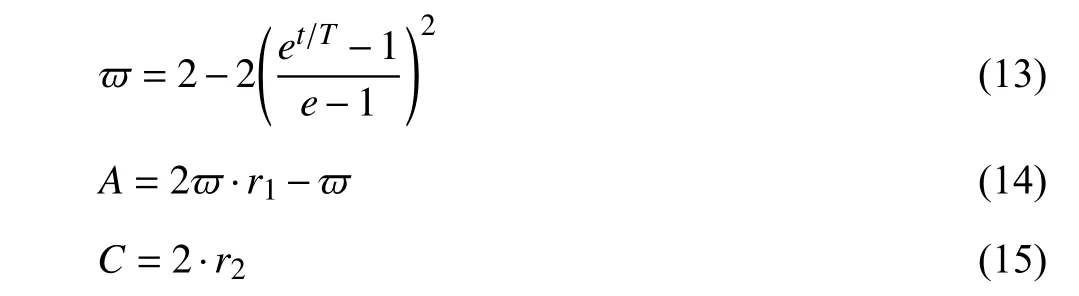
where t is the current number of iterations, and r1and r2are the random vectors between [0,1].

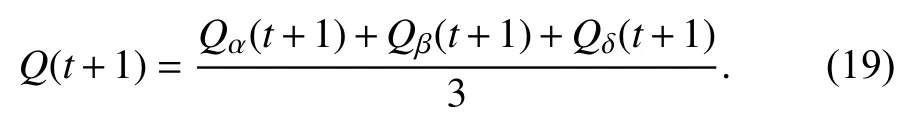
Step 5: Update the positions of the three best wolves by

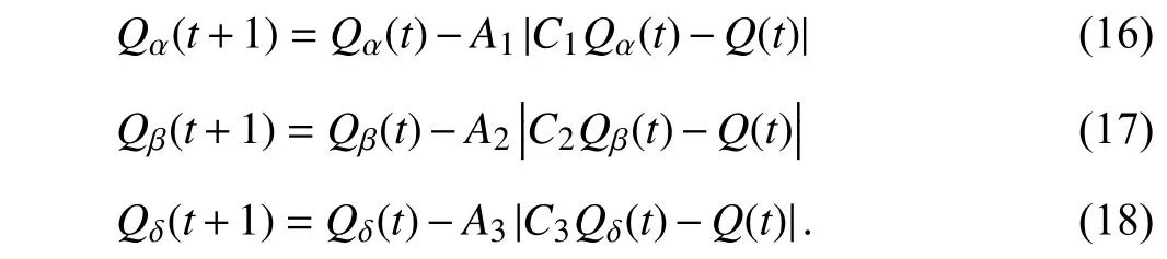
Step 6: Update the individual position by

Step 7: Terminate the algorithm if the termination criterion is reached and output the optimal individual position.Otherwise, go back to Step 3 and continue the algorithm.

E. Online RUL Estimation

The well-trained SVR and LSTM models together with the obtained optimal connection parameters ( w1, w2, and b) can result in a high-performance hybrid model, which will be used to predict the RUL online. With the online monitoring data of an in-service system, we seek to predict how long the system can be operated safely, that is, to predict the time span between the current moment and the future true system failure moment.

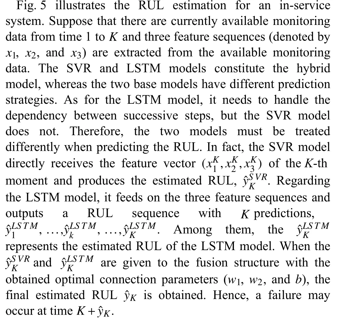
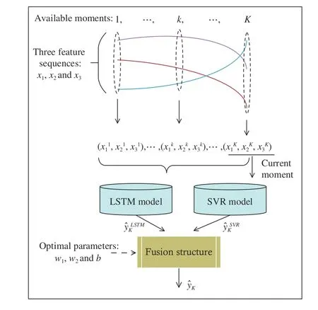
Fig.5. Illustration of RUL estimation for an in-service system.

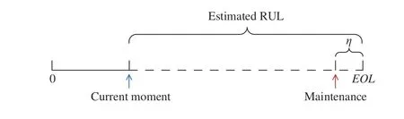
Fig.6. Illustration of maintenance scheduling.

There are two possible scenarios in real-world maintenance activities. If the scheduled preventive maintenance moment is conducted earlier than the actual failure moment of the inservice system, the preventive maintenance is effective. On the other hand, if the in-service system fails earlier than the scheduled preventive maintenance moment, the preventive maintenance is void and corrective maintenance must be taken.

The maintenance cost rate (MCR), defined as the ratio between the total maintenance cost and total life cycle duration, can be used to estimate the performance of the RUL estimation. The estimated RUL with lower MCR is considered to have better performance. It intends to measure the benefit provided by risk-averse prognostics. When the in-service system still works but the preventive maintenance is performed, the MCR is given by

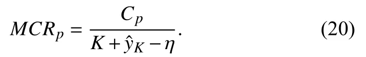
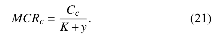
On the other hand, if the system fails, corrective maintenance must be carried out. In this event, the total maintenance cost is Ccand the total life cycle duration is K+y. Thus, according to the definition of MCR, the MCR of the corrective maintenance is given by

In general, the prediction accuracy of a model is between 50% and 100%. The 100% prediction accuracy means perfect prognostics, whereas the 50% prediction accuracy implies unsatisfactory prediction results. In this sense, the estimated failure time in (20) is supposed to satisfy 0.5(K+y)≤K+yˆK≤K+y. Thus, for the ideal PdM case with perfect prognostics,the MCR becomes

It is worth noting that the ideal PdM case is only an ideal hypothesis which cannot be achieved in practice. However,the MCRidealcan help understand the gap between reality and ideal. In addition, this inequality, 0.5(K+y)≤K+yˆK−η, can also be satisfied considering that the time margin η is usually small. As mentioned before, the corrective maintenance is more expensive than the preventive maintenance and this means that Cc>2Cpis reasonable. Through 0.5(K+y)≤K+yˆK−η and Cc>2Cp, one can get (Cc)/(K+y)>(Cp)/(K+yˆK−η). Therefore, the proposed cost metric tends to favor lead prediction. In other words, the overestimated RUL will be more costly than the underestimated RUL.

IV. VERIFICATION

A. Dataset Description

To verify the performance of the proposed risk-averse RUL estimation method and the PdM strategy, a turbofan engine degradation simulation dataset [34] is considered. The dataset consists of multivariate time series signals generated by CMAPSS. Fig.7 shows a sketch of the main components of the turbofan engine, including the fan, low-pressure compressor(LPC), high-pressure compressor (HPC), high pressure turbine(HPT), and low pressure turbine (LPT). A total of 21 signals that can describe the degradation process were generated, as shown in Table I. The first nine signals were obtained by direct measurement of Sensors 1–9, while the rest were gained by soft measurement of Sensors 10–21 [35].

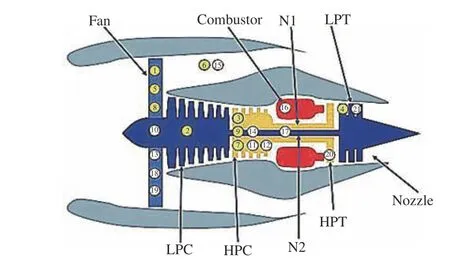
Fig.7. Sketch of the main components of the engine [35].

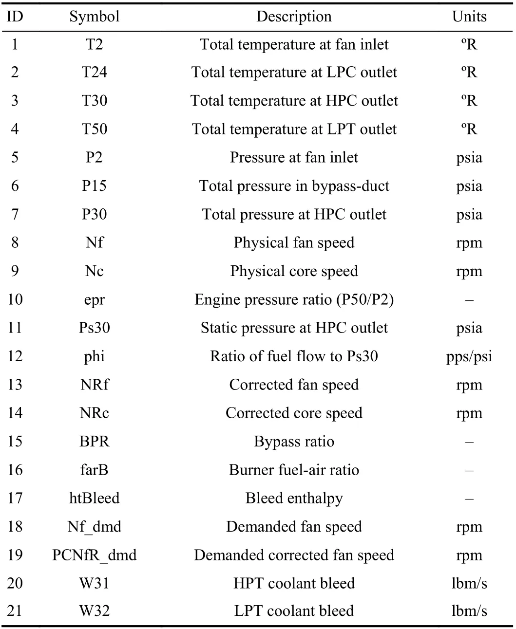
TABLE I DESCRIPTION OF THE SENSOR DATA [35]

Dataset “FD001” is used in this paper. It describes the gradual degradation process of HPC under one failure mode and one operating condition. The dataset contains three.txt files: “train_FD001.txt”, “test_FD001.txt” and “RUL_FD001.txt”. “train_FD001.txt” records the complete life cycles of 100 engines from the beginning to failure, “test_FD001.txt” is composed of 100 incomplete time series ending up prior to failure, and “RUL_FD001.txt” provides the actual RUL values.

B. RUL Estimation Results

Based on the provided dataset, the first step is to extract the degradation features of the engines. According to Section III-B,the moving average technique is utilized for tendency extraction, and the moving window size n is set to 20. Next,the correlation and consistency indicators of each sensor are calculated using (2) and (3), as shown in Table II. In this paper, the sensor with absolute value of correlation indicator greater than 0.7 is regarded as a stronger linear correlation.Thus, the sensors that satisfy |Corr|≥0.7 and Con=0 or 1 will be selected.

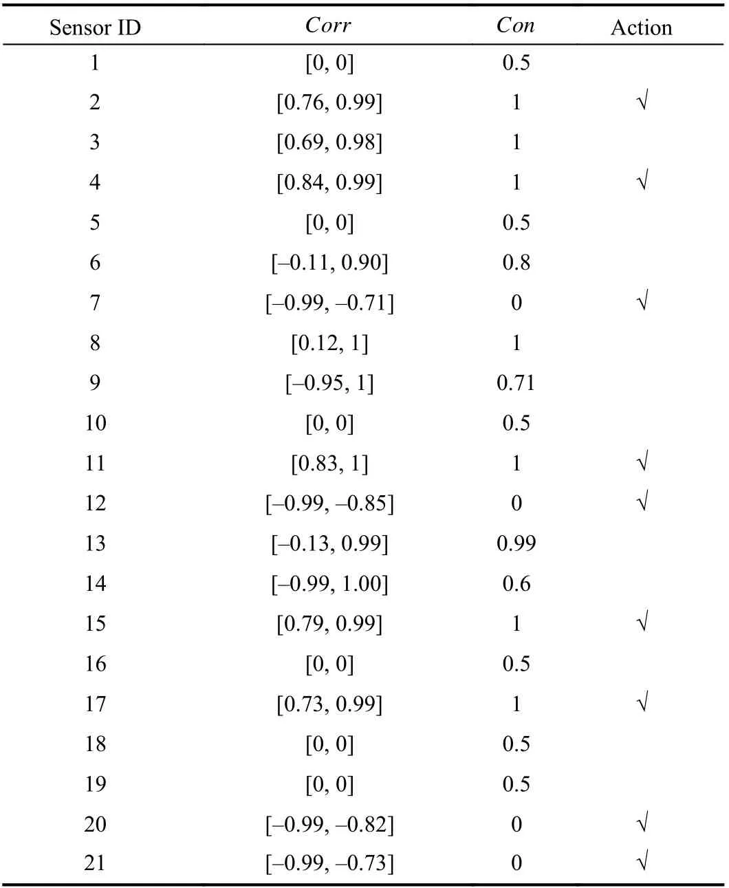
TABLE II CORRELATION AND CONSISTENCY INDICATORS FOR 21 SIGNALS

Considering that sensors 1, 3, 5, 6, 8, 9, 10, 13, 14, 16, 18,and 19 do not meet the limitation of the correlation indicator,they will be eliminated. Subsequently, the remaining sensors will be tested by the consistency indicator. These sensors that have passed the test will be maintained. Thus, the remaining nine sensors are selected, i.e., the sensors 2, 4, 7, 11, 12, 15,17, 20, and 21.

With the obtained degradation features, the SVR and LSTM models are separately trained to establish the nonlinear mapping relationship between the features and the RUL. In this experiment, the number of hidden units, learning rate, and dropout probability of the LSTM model are specified as 200,0.01, and 0.5, respectively. The SVR hyper-parameters, such as box constraint, Gaussian kernel scale parameter and ε, are set to 1, 1, and 0.1, respectively.

Considering that the degradation of the engine is usually not noticeable before running for a while, this means it may not be reasonable to estimate the RUL at this stage [36]. Thus, this paper clips the responses at the RUL threshold 150, which is determined via several trials with best performance on the test dataset. That is to say, the models will treat the instances with higher RULs as equal, which enables the models to learn more essential mapping relationship when the engines are close to failing. Fig.8 shows the parts of prediction results on the test set.

For the test engines ID 31 and ID 38, the predicted values of the LSTM model are closer to the actual values than those of the SVR model. However, for test engine ID 78, the SVR model outperforms the LSTM model. Besides, it is observed from the test engine ID 91 that the prediction curve of the LSTM model is approaching the actual curve prior to Cycle 155.After that, the SVR model has the upper hand. These results indicate that each of the studied SVR and LSTM models has its own benefits and drawbacks, and there is no clear-cut winning method. Nevertheless, it must be pointed out that late prediction is intolerable. For example, there are obvious late predictions for the test engine ID 78, and the consequences of the late predictions may be catastrophic. Therefore, the riskaverse adaptation is necessary, and the next section will present the verification results for the risk-averse RUL estimation.

C. Risk-Averse RUL Estimation Results on Test Data

The GWO-II algorithm is used to determine the values of w1, w2, and b. To enable the GWO-II algorithm to reach a convergence state, the population size is set to 20 and the maximum number of iterations is set to 50. The search spaces of the three parameters are set between −10 and 10. Also, the corrective maintenance cost and preventive maintenance cost are assumed to be 500 and 100, respectively. Generally speaking, it is difficult to describe a four-dimensional space,such as w1, w2, b, and z. For visualization, the threedimensional view of w1, w2, and z is depicted in Fig.9. This figure shows the distribution of the grey wolf population during the optimization process.

In the initial stage, the grey wolves are randomly distributed in the space. Through the surrounding, hunting, and attacking operations, the grey wolf population is able to obtain the information about the prey (optimal solution) [37]. Thus, as the number of iterations increases, the grey wolves gradually gather into the optimal solution area. At the 30th iteration, the GWO-II algorithm finds the optimal solution, that is w1=0.22, w2=0.89, and b=−0.05.

With the obtained values of w1, w2, and b, the hybrid model is used to estimate the RULs on the test set. Fig.10 shows the estimated RUL results on 100 test samples using the hybrid model. It is observed that the estimated values can not only follow the changes in actual values but also approach the actual ones. This implies that the use of the hybrid model is feasible to predict the RULs.

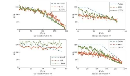
Fig.8. Prediction results on several test samples.

Fig.9. Search process of GWO-II algorithm for parameters w1 and w2.

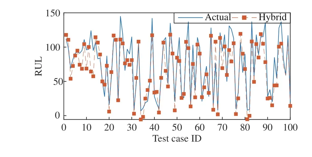
Fig.10. Estimated RUL results for 100 test samples.

Fig.11 shows the distribution of errors for SVR, LSTM and hybrid models. The prognostics on the left side of the red dotted line refers to the lead prediction. It is obvious that the hybrid model has more lead predictions compared with the SVR and LSTM models. Specifically, the numbers of lead predictions for SVR, LSTM, and hybrid models are 40, 44,and 70, respectively. The results imply that both SVR and LSTM models tend to late predictions. However, as mentioned before, such late predictions are intolerable due to the potential for catastrophic consequences. Unlike the simple SVR or LSTM models, their combination gives good results.This should be attributed to the fusion structure proposed in Section III-C and the penalty mechanism proposed in Section III-D.

It should be pointed out that the lead prediction without considering the prediction error is meaningless. Thus, the root mean square errors (RMSEs) of the three models are calculated and shown in Fig.11. The RMSE of the hybrid model is 19.11, which is lower than 24.61 of the SVR and 20.16 of the LSTM, indicating that the hybrid model is superior in prediction precision as well. To sum up, the lead prediction number and the prediction precision of the hybrid model meet the expected goal, which is to reduce the over estimation rate while maintaining a reasonable under estimation level, showing that the proposed risk-averse RUL estimation approach is effective.

D. Performance Evaluation

In this section, the proposed RUL estimation method will be evaluated from the perspective of predictive maintenance.According to the maintenance scheduling in Section III-E, as an illustration, Table III gives the maintenance cost rates of three RUL prognostic strategies for test engines ID 1–10.Here, “Tm” denotes the planned maintenance moment, “P”indicates that the maintenance action taken (MAT) is preventive maintenance, and “C” indicates that the MAT is corrective maintenance. The time margin of the reliability, η,is considered as 10.

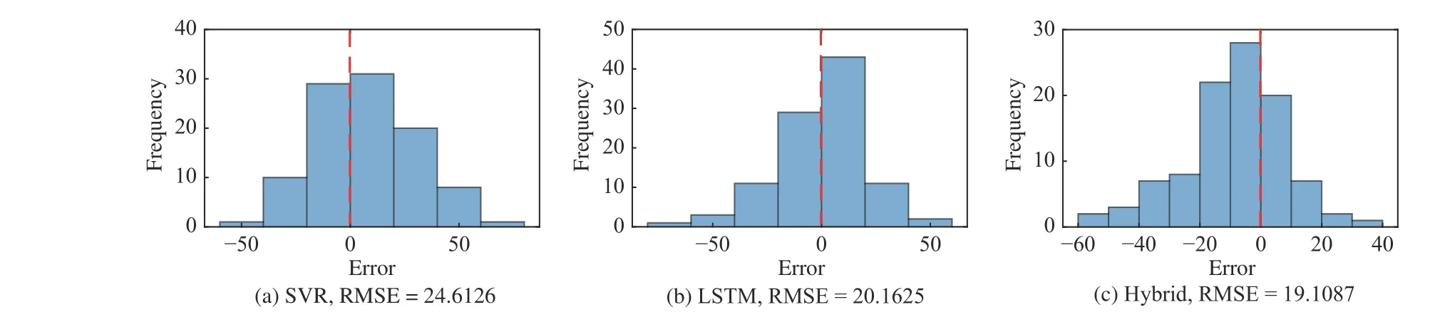
Fig.11. Distribution of errors for SVR, LSTM and hybrid models.

TABLE III MAINTENANCE COST RATES FOR TEST ENGINES ID 1–10

From the given MCRs, it is obvious that the corrective maintenance is more costly than the preventive maintenance.From the maintenance activities taken, the use of hybrid model, instead of the SVR or LSTM model, allows improving the accuracy of maintenance decisions. For example, for the test engines ID 1, 6, and 7, the scheduled maintenance actions using SVR model are unreasonable. The similar situation can be found in the LSTM model, such as the test engines ID 1, 2,6, and 9. Best of all, the use of hybrid model leads to correct the maintenance decisions for the test engines ID 1, 6, 7, and 9, which is significant for ensuring the operation safety and reliability of the engines. Besides, it is observed that the MCR of the hybrid model is sometimes higher than that of SVR and LSTM models under the preventive maintenance, but it is allowable compared with the corrective maintenance.

The MCRs for the 100 test samples can be visualized in Fig.12. The test samples are divided into five groups, and each group has 20 engines. The average MCR of each group is calculated based on different prognostic approaches (SVR,LSTM, hybrid models, and ideal PdM case). Evidently, no matter which group, the average MCR of the hybrid model is lower than those of the SVR and LSTM models. Based on this, the average MCRs of the four prognostic approaches for all test samples are calculated. In detail, the average MCR for the SVR model is 1.49, 1.20 for the LSTM model, 0.80 for the hybrid model and, 0.50 for the ideal PdM case. Compared with the SVR and LSTM models, the average MCR of the hybrid model is reduced by 46.44% and 33.41%, respectively.Also, there is only a MCR gap of 0.3 between the hybrid model and the ideal model. These results show that the benefits the risk-averse RUL estimation brings are considerable, and the proposed approach can significantly reduce the maintenance cost rate and is approaching the ideal one.

Fig.12. MCRs for 100 test samples using SVR, LSTM and hybrid models.

V. CONCLUSIONS

In this work, an RUL estimation method with risk-averse adaptation has been proposed. It hybridizes two mainstream models, SVR and LSTM, in the field of RUL prognosis. The proposed estimation method can enhance the robustness of prediction, increase the marginal utility, and reduce the overestimation rate while maintaining a reasonable under estimation level. Besides, an embedded degradation feature selection module can obtain crucial features that reflect system degradation trends, and a proposed maintenance cost rate can measure the benefit provided by risk-averse prognostics.

The verification results using NASA data repository reveal the feasibility and effectiveness of the proposed method.According to the number of lead predictions, the prediction errors, the accuracy of maintenance decisions, and the maintenance cost rate, the proposed hybrid model is indeed better than the single models. Above all, the precise and riskaverse RUL estimation is significant for a system to keep safe and stable operation.

The proposed method can also be applied to other engineering systems subjected to single failure modes.Considering that the failure of some engineering systems may be caused by coupling actions of various failure modes, our future work will focus on the investigation of the systems with multiple failure modes.