Fixed Point Theory and the Existence of Two Positive Periodic Solutions of Riccati’s Equation

NI Hua(倪华)

(School of Mathematical Science,Jiangsu University,Zhenjiang 212013,China)

Abstract: This paper deals with a class of Riccati’s equation.By the principle of contraction mapping,the existence of one positive periodic solution of Riccati’s equation is obtained;By variable transformation method,Riccati’s equation is turned into Bonulli’s equation.According to the periodic solution of Bernoulli’s equation and variable transformation,another periodic solution of Riccati’s equation is obtained.And we discuss the stability of the two positive periodic solutions,one periodic solution is attractive on some region and unstable on another region,and another periodic solution is unstable on R.

Key words: Riccati’s equation;Contraction mapping;Periodic solution;Stability

1.Introduction

Consider the nonlinear Riccati type first-order differential equation：

No matter in the classical theory of differential equation or in the branches of modern science,Riccati’s equation has important applications,and there are many studies on this equation[1−6].In [1-2],the sufficient conditions of the existence of periodic solutions of Eq.(1.1)were given,also in [1],the stability of periodic solutions of Eq.(1.1)was obtained;In[3],the author studied some special types of Riccati’s equation,and got the general solution and periodic solutions of Eq.(1.1);In [4],the author discussed Eq.(1.1)with characteristic multiplier;In[5],the author considered the high dimensional Riccati’s equation,and obtained some sufficient conditions of the existence of periodic solutions of Eq.(1.1);In [6],the author got some criteria for the existence of periodic solutions of Eq.(1.1).

Recently,Mokhtarzadeh,Pournaki and Razani[7]dealed with scalar Riccati’s differential equations,and assumed that a,b,and c areω-periodic continuous real functions on R and gave certain conditions to guarantee the existence of at least one periodic solution for Eq.(1.1);Wilczynski[8]gave a few sufficient conditions for the existence of two periodic solutions of the Riccati’s ordinary differential equation in the plane.

However,the above literatures only give the existence of periodic solutions,but few papers involve the size range and stability of periodic solutions.Whenb(t)≡0,in [9],we abtain the existence of two periodic solutions Riccati’s equation withω-periodic coefficients and different symbols.One of these solutions is unstable on R and the other one is attractive on some region.

In this paper,we discuss a class of Riccati’s equation.By the principle of contraction mapping and variable transformation method,we obtain the existence of two positive periodic solutions of Riccati’s equation,and give the ranges of the size of the periodic solutions;further,we discuss the stability of the two periodic solutions.One periodic solution is attractive on a certain region and unstable on another region,and another periodic solution is unstable on R.Some conclusions of related papers (e.g.[1,9])are generalized.

2.Preliminaries

In this section,we give a lemma which will be used later.

Lemma 2.1[10]Consider the following:

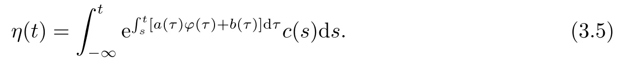
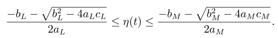
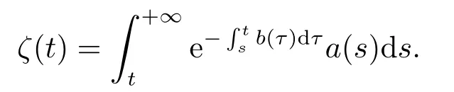
wherea(t),b(t)areω-periodic continuous functions on R.Ifthen Eq.(2.1)has a uniqueω-periodic continuous solutionη(t),andη(t)can be written as follows:

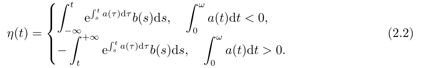
For the sake of convenience,suppose thatf(t)is anω-periodic continuous function onR.We denote

The rest of the paper is arranged as follows:We will study the existence and stability property of the periodic solutions of Eq.(1.1)in the next section,we end this paper with two examples.

3.Existence and Stability of the Periodic Solutions

In this section,we obtain the existence of periodic solutions of Riccati’s equation by using the contraction mapping theorem,and discuss the stability of periodic solutions.Moreover,this proof process is suitable for a class of Bernoulli’s equation,so we can get the existence and stability of periodic solutions of the class of Bernoulli’s equation.

Theorem 3.1Consider Eq.(1.1),a(t),b(t)andc(t)are allω-periodic continuous functions on R.Suppose that the following conditions hold:

(H1)a(t)>0;

(H2)b(t)<0;

(H3)c(t)≥0;(c(t)0);

(H4)b2M −4aMcM >0.

Then Eq.(1.1)has two positiveω-periodic continuous solutions:

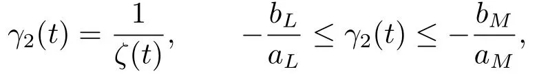
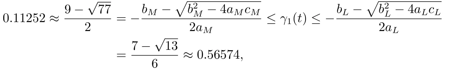
1)One positiveω-periodic continuous solution isγ1(t),

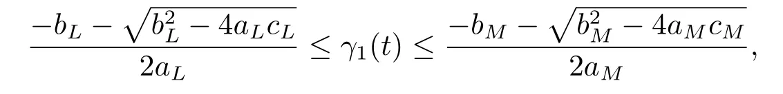
andγ1(t)is attractive if given initial value onand unstable if given initial value onHerex(t0)is any given initial value of Eq.(1.1),and

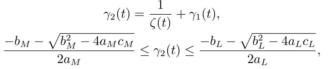
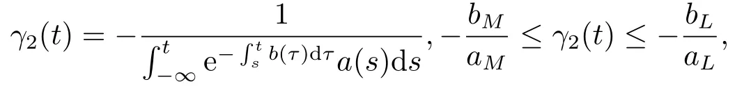
2)Another positiveω-periodic continuous solution isγ2(t),

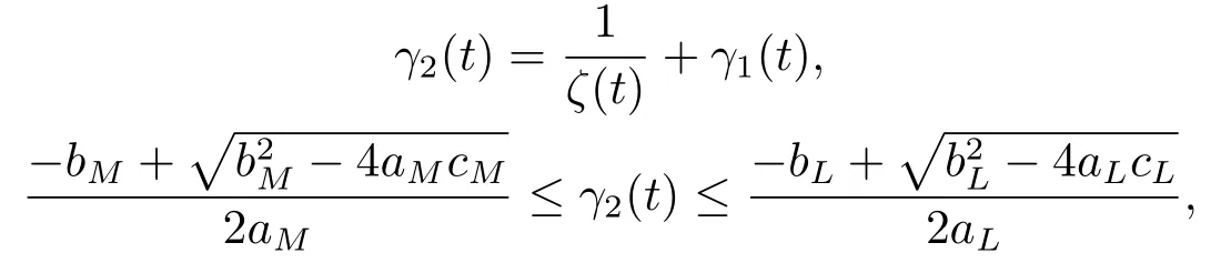
andγ2(t)is unstable on R.

Proof1)We prove that Eq.(1.1)has two positiveω-periodic continuous solutionsγ1(t)andγ2(t).

Define a set as follows:

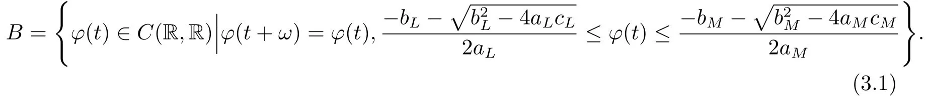
By (H1),(H2),(H3)and (H4),we have

ThusB∅,given anyφ(t),ψ(t)∈B,the distance is defined as follows:

Thus (B,ρ)is a complete metric space.

Given anyφ(t)∈B,consider the following equation:

Sincea(t),b(t),c(t)andφ(t)areω-periodic functions on R,anda(t)φ(t)+b(t)is anω-periodic function on R,by (3.1),(H1)and (H2),we get that

Hence we have

According to Lemma 2.1,Eq.(3.3)has a uniqueω-periodic continuous solution as follows:

By (H3),(3.4)and (3.5),we get

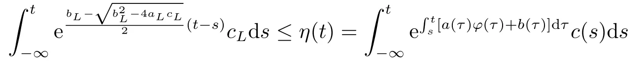
Thus we have

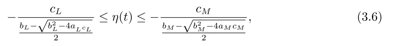
that is,

Hence,η(t)∈B.

Define a mapping as follows:

Thus if given anyφ(t)∈B,then (Tφ)(t)∈B.HenceT:B →B,Given anyφ(t),ψ(t)∈B,we have

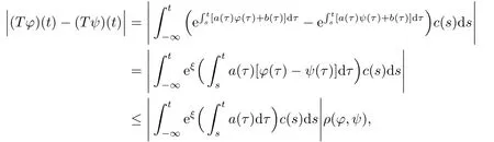
here,ξis betweendτ.By (3.4),it follows

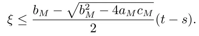
Hence we have

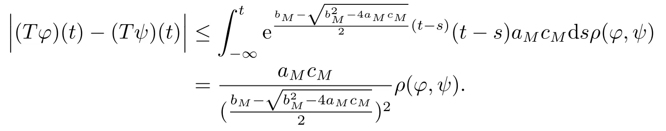
Therefore,we can get

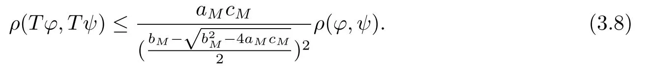
By (H2)and (H4),it follows

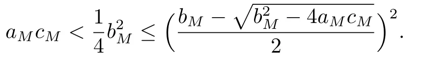
Hence we have

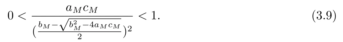
By (3.8)and (3.9),Tis a contraction mapping.According to the contraction mapping principle,Thas a fixed point onB.The fixed point is the positiveω-periodic continuous solutionγ1(t)of Eq.(1.1),and

Let

herex(t)is the unique solution of Eq.(1.1)with initial valuex(t0)=x0,andγ1(t)is the periodic solution of Eq.(1.1).Differentiating both sides of(3.11)along the solution of Eq.(1.1),we get

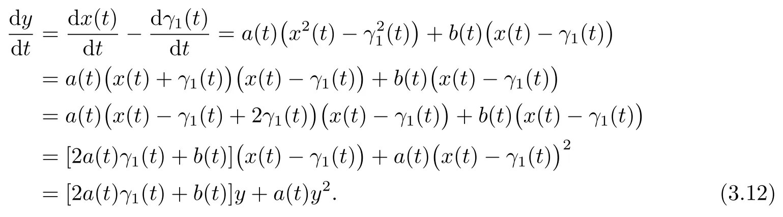
This is Bernoulli’s equation.Let

then Eq.(3.12)can be turned into the following equation:

Note that

thus we have

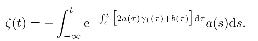
According to Lemma 2.1,Eq.(3.14)has a uniqueω-periodic continuous solution as follows:

By the transformations (3.11)and (3.13),it follows that Eq.(1.1)has anotherω-periodic continuous solutionγ2(t)as follows:

Suppose thatt∗is the extreme point of functionγ2(t),then we have

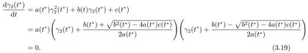
Then we can get that all extreme pointst∗of functionγ2(t)satisfy

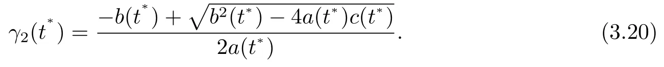
Thus we have

2)We prove the stability of two periodic solutionsγ1(t)andγ2(t)of Eq.(1.1).

Firstly,we prove the stability of the periodic solutionγ1(t)of Eq.(1.1).

Easy to know,the unique solutionu(t)of Eq.(3.14)with initial valueu(t0)=u0is as follows:

By (3.11)and (3.13),the initial valueu(t0)=u0can be written as follows:

thusu(t)can be rewritten as follows:

By (3.13),it follows

By (3.11),we have

By (3.16),it follows

Therefore,theω-periodic solutionγ1(t)of Eq.(1.1)is attractive if given initial valuex(t0)∈

(ii)If

by (3.17),(3.28),(3.30)and (3.25),we have

Under the condition of (3.30),now,we discussu(t0)in two cases.

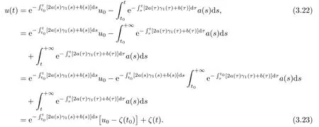
From (3.32),(3.22),whent>t0,it follows

By (3.31),(3.33)and (3.27),we have

Thus theω-periodic solutionγ1(t)of Eq.(1.1)is attractive if given initial value

By(i)and(I)of(ii),theω-periodic solutionγ1(t)of Eq.(1.1)is attractive if given initial value

Thusu(t0)=>0.Combined by (3.31),according to zero point theorem,there exists at∗>t0,such that

Therefore,whent →t∗,we have

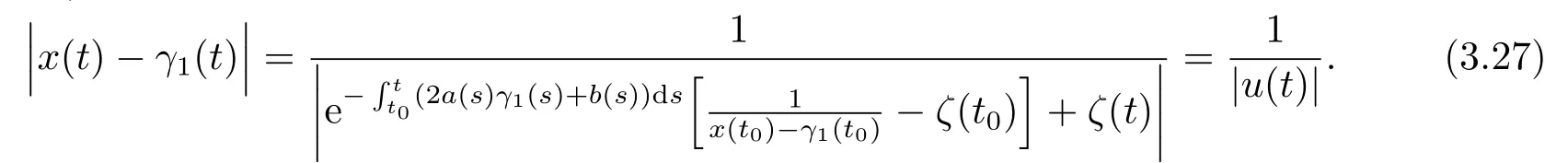
By (3.27)and the formula above,it follows

Combining (3.30)and (3.37),we can get

By (II)of (ii),the periodic solutionγ1(t)of Eq.(1.1)is unstable if given initial value

Thus by (II)of (ii)and (iii),we get that if given initial value

γ1(t)is unstable.

Next,we prove the stability of the periodic solutionsγ2(t)of Eq.(1.1).

By (3.18),it follows

herex(t)is the unique solution of Eq.(1.1)with initial valuex(t0)=x0.From the above proof,by (3.29),we know,whenx(t0)∈D1,that is to say,given anyε >0,there is aT >0,such thatSo,whent ≥t0+T,we have

Because of the arbitrariness ofε,it follows

Note thatζ(t)is bounded and positive on R,thusγ2(t)is unstable ifx(t0)∈D1.

Whenx(t0)∈D2,by (3.39),there exists at∗>t0,such that

Sinceζ(t)is bounded and positive on R,we have

Thusγ2(t)is unstable ifx(t0)∈D2.

Therefore,theω-periodic solutionγ2(t)of Eq.(1.1)is unstable onD1∪D2=R.

This is the end of the proof of Theorem 3.1.

Theorem 3.2Under the conditions of Theorem 3.1,Eq.(1.1)has exactly twoω-periodic continuous solutions:γ1(t)andγ2(t).

ProofThe proof of the existence ofγ1(t)andγ2(t)is given in Theorem 3.1.Now,we prove that Eq.(1.1)has exactly twoω-periodic continuous solutions:γ1(t)andγ2(t).

We know ifx(t0)=γ1(t0),the unique solution of Eq.(1.1)isγ1(t),and ifx(t0)=γ2(t0)=the unique solution of Eq.(1.1)isγ2(t).

(i)Ifx(t0)>γ2(t0)=by(3.46),the unique solutionx(t)of Eq.(1.1)satisfies

Thusx(t)can not be a periodic solution.

Hencex(t)can not be a periodic solution.

Therefore,Eq.(1.1)has exactly twoω-periodic continuous soluctions:γ1(t)andγ2(t).

This is the end of the proof of Theorem 3.2.

Remark 3.1From the proof of Theorem 3.1,ifc(t)≡0,(3.9)is not satisfied,butTalso has a fixed point onB.The fixed point onBis the periodic solutionγ1(t)= 0,thus ,it is easy for us to draw the following corollary on Bernoulli’s equation.

Corollary 3.1Consider the following Bernoulli’s equation:

anda(t),b(t)are bothω-periodic continuous functions on R.Suppose that the following conditions hold:

(H5)a(t)>0;

(H6)b(t)<0.

Then Eq.(3.47)has exactly twoω-periodic continuous solutions:

1)Oneω-periodic continuous solution isγ1(t)=0,andγ1(t)is attractive if given initial value onand unstable if given initial value onherex(t0)is any given initial value of Eq.(3.47),and

2)Anotherω-periodic continuous solution isγ2(t),

andγ2(t)is unstable on R.

Theorem 3.3Consider Eq.(1.1),a(t),b(t)andc(t)are allω-periodic continuous functions on R.Suppose that the following conditions hold:

(H7)a(t)<0;

(H8)b(t)>0;

(H9)c(t)≤0;(c(t)0);

(H10)b2L −4aLcL >0.Then Eq.(1.1)has two positive continuousω-periodic solutions.

1)One positiveω-periodic solution isγ1(t),

andγ1(t)is unstable on R;

2)Another positiveω-periodic solution isγ2(t),

andγ2(t)is attractive if given initial value onand unstable if given initial value onherex(t0)is any given initial value of Eq.(1.1),and

ProofConsider the following equation:

Theorem 3.4Under the conditions of Theorem 3.3,Eq.(1.1)has exactly twoω-periodic continuous solutions:γ1(t)andγ2(t).

ProofTheorem 3.4 also follows by applying Theorem 3.2 to the equation (3.48).

Similar to Corollary 3.1,we have

Corollary 3.2Consider Bernoulli’s Eq.(3.47),anda(t),b(t)are bothω-periodic continuous functions on R.Suppose that the following conditions hold:

(H11)a(t)<0;

(H12)b(t)>0.Then Eq.(3.47)has exactly twoω-periodic continuous solutions:

1)Oneω-periodic continuous solution isγ1(t)=0,andγ1(t)is unstable on R;

2)Anotherω-periodic continuous solution is andγ2(t)is attractive if given initial value onand unstable if given initial value onherex(t0)is any given initial value of Eq.(3.47).

4.Examples

The following examples show the feasibility of our main results.

Example 4.1Consider the following equation:

It is easy to calculate thataM=3,aL=1,bM=−7,bL=−9,cM=3,cL=1,and

Clearly,the conditions (H1)-(H4)of Theorem 3.1 are satisfied.It follows from Theorem 3.1 that Eq.(4.1)has two positive 2π-periodic continuous solutionsγ1(t)andγ2(t),and

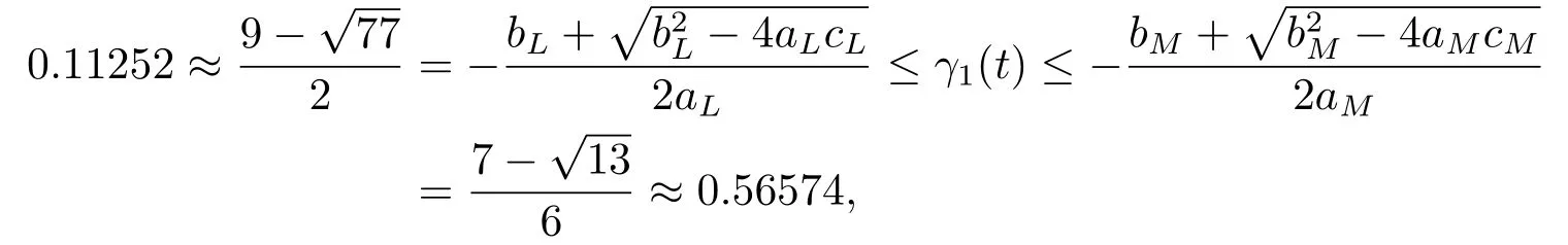
andγ1(t)is attractive onand unstable on

herex(t0)is any given initial val ue of Eq.(4.1),and

Another 2π-periodic continuous solution isγ2(t),

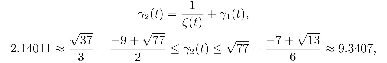
andγ2(t)is unstable on R.

From this example,using matlab,we can deduce the value 3.541<γ2(0)=+γ1(0)<3.542.When initial valuex(0)≤3.541,the solution curve of Eq.(4.1)tends to the curve of the periodic solutionγ1(t)astachieves at some value (see Fig.4.1);When initial valuex(0)≥3.542,the solution curve of Eq.(4.1)arrives at enough large (+∞)at some timet∗(see Fig.4.2).

Example 4.2Consider the following equation:

It is easy to calculate thataM=−1,aL=−3,bM=9,bL=7,cM=−1,cL=−3,and

Clearly,the conditions (H7)-(H10)of Theorem 3.3 are satisfied.It follows from Theorem 3.3 that Eq.(4.2)has two positive 2π-periodic continuous solutionsγ1(t)andγ2(t),and

andγ1(t)is unstable on R.

Another 2π-periodic continuous solution isγ2(t),

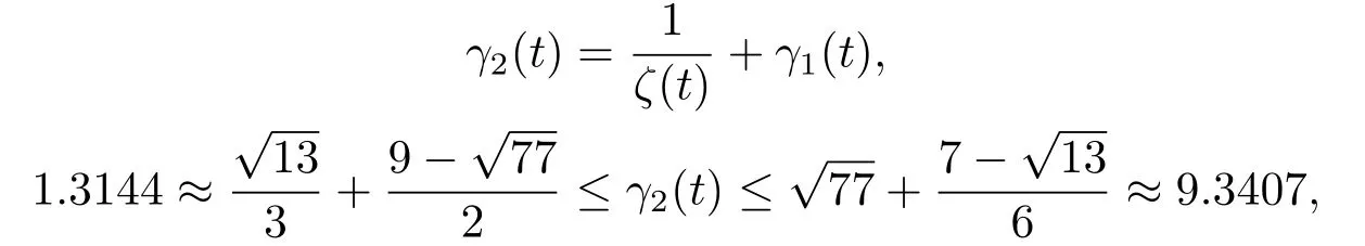
andγ2(t)is attractive onD1={x(t0)|x(t0)>γ1(t0)},and unstable onD2={x(t0)|x(t0)≤γ1(t0)},herex(t0)is any given initial value of Eq.(4.2),and

From this example,using matlab,we can deduce the value 1.28<γ1(0)<1.29.When initial valuex(0)≥1.29,the solution curve of Eq.(4.2)tends to the curve of the periodic solutionγ2(t)astachieves at some value (see Fig.4.3);When initial valuex(0)≤1.28,the solution curve of Eq.(4.2)arrives at enough large (−∞)at some timet∗(see Fig.4.4).

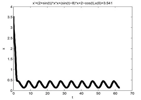
Fig.4.1 The curve of the solution of Eq.(4.1)with initial value x(0)=3.541

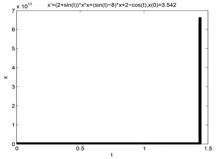
Fig.4.2 The curve of the solution of Eq.(4.1)with initial value x(0)=3.542

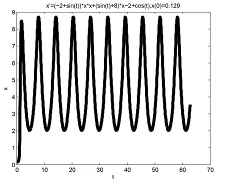
Fig.4.3 The curve of the solution of Eq.(4.2)with initial value x(0)=0.129

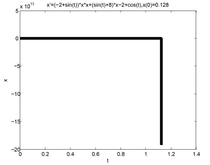
Fig.4.4 The curve of the solution of Eq.(4.2)with initial value x(0)=0.128