Model predictive inverse method for recovering boundary conditions of two-dimensional ablation∗

Guang-Jun Wang(王广军), Ze-Hong Chen(陈泽弘), Guang-Xiang Zhang(章广祥), and Hong Chen(陈红),†

1School of Energy and Power Engineering,Chongqing University,Chongqing 400044,China

2Key Laboratory of Low-grade Energy Utilization Technologies and Systems,Ministry of Education,Chongqing University,Chongqing 400044,China

Keywords: ablation,heat transfer,model predictive inverse method(MPIM),boundary reconstruction

1. Introduction

Measurement of time- and space-dependent heat flux is widely carried out in numerous engineering applications,such as aerospace industry,[1-4]metallurgy industry,[5,6]combustion diagnosis,[7,8]and biomedical engineering.[9,10]Direct measurement of transient heat flux is often difficult in many industry fields,such as the heat flux on thermal protection shield surface of the re-entry vehicle,and the cooling heat flux on the casting surface that determines the casting quality of continuous casting process. For these circumstances, with the idea of inverse analysis,the time-and space-dependent heat flux is able to be indirectly obtained by solving inverse heat transfer problems(IHTPs).

The core of the above indirect measurement is to solve an inverse problem which is commonly ill-posed.[11-15]Thus, various optimization methods with anti-ill-posedness are developed. Heuristic algorithms[7,16-19]and gradient algorithms,[20-22]as the typical inverse methods, are widely used to solve the inverse problems. For the IHTPs,Vakili and Gadala[23]used particle swarm optimization(PSO)algorithm to estimate the boundary conditions with different dimensions.Sun et al.[24]introduced sequential quadratic programming(SQP) algorithm to retrieve the transient heat flux of participating media. Tapaswini et al.[25]used a variational iteration method(VIM)to reconstruct the boundary heat flux. Sun et al.[26]employed the decentralized fuzzy inference method(DFIM)to estimate the time-and space-dependent heat flux of two-dimensional(2D)participating medium.

The above researches all focused on estimating the transient heat flux of the systems with fixed boundary. For the IHTPs with the ablation of the thermal protection shield of reentry vehicle, the transient heat flux on the ablated surface is more difficult to reconstruct. The reason is that the boundary of the system will move due to the phase change on the ablation material surface. Several researches have been achieved in the ablation inverse problems. de Oliveira et al.[27]used the conjugate gradient method (CGM) to recover the functional form of the heat flux on the ablated surface of one-dimensional(1D)slab. Molavi et al.[28]developed one CGM with the first order Tikhonov regularization to estimate the surface recession and the time-varying net heat flux on the ablated surface of 1D slab. In the above researches,the conjugate gradient algorithms were used to simultaneously estimate the unknown heat flux on the whole-time domain with the temperature measurements. Therefore, the estimation result could not be obtained in real time. In order to estimate the heat flux online,Mohammadiun et al.[29]and Farzan et al.[30]used the sequential function specification method (SFSM) to sequentially reconstruct the surface heat flux of 1D ablation in time domain.Although the SFSM is able to solve the inverse problem in real time, the accuracy of the solution obtained by the SFSM significantly depends on the number of future time steps. In addition,it is necessary that the specific function of unknown parameter over a period of future time should be assumed in advance.[14]

Most of previous studies described the ablation process as 1D problem. However, the surface heat flux of the ablation material has obvious unevenness in space, and the ablation velocity obviously presents spatial difference.[31]Therefore, the ablation process is multi-dimensional, in which the surface heat flux is time-and space-dependent and the temperature field is more complex. Considering the characteristics,for the ablation process, multi-dimensional ablation inverse method should be established. Moreover, developing a more efficient method is an urgent requirement for addressing the sort of IHTP.

Based on the dynamic matrix control (DMC), an inverse method for the unsteady heat conduction problem was established.[32-34]This inverse method can effectively reduce the sensitivity of the estimation result to the temperature measurement errors and the dependence of the accuracy on the number of future time steps.

In this paper,a model predictive inverse method(MPIM)is presented to estimate the time- and space-dependent heat flux and the ablation velocity on the ablated boundary of a 2D ablation process. In Section 2, a heat transfer model of the 2D ablation process is described and one numerical simulation technique for the ablation process is introduced. In Section 3, the inverse problem of the 2D ablation process is established and the corresponding MPIM is introduced in detail. In Section 4, the transient heat flux distribution on the ablated boundary is estimated. In addition,the effects of temperature measurement errors,the number of future time steps and arrangement of measurement points on the reconstruction results are studied in this section. In Section 5,the main conclusions are drawn.

2. Ablation model and numerical method

2.1. Ablation model

For a 2D ablation system shown in Fig.1, the ablation material is heated by the time-and space-dependent heat flux on a boundary.In the figure,q(x,t)is the total heat flux,which brings about the complex thermal action on the heated boundary. The thermal action contains the conduction heat,radiative heat transfer, the heat fluxes generated by complex physical and chemical processes, etc.[35,36]Complete ablation process goes through a heat conduction stage and an ablation stage.At the beginning,the temperature of the heated boundary does not reach the phase transition temperature TABof the ablation material,so that the total heat flux q(x,t)exerted on the boundary only enters into the interior of the material through heat conduction. As the heating continues, temperatures of some locations on the heated boundary reach TAB,which causes the boundary recession.During the ablation stage,part of q(x,t)is converted into the heat flux of material vaporization qdthat is dissipated into the environment and the remaining heat flux qcenters into the interior of the material through heat conduction.

For studying the ablation heat transfer process, the following simplifications are considered, as suggested in Ref. [37]: (i) during the ablation stage, the ablation material gasifies directly without going through the liquefaction process; (ii) the heat absorbed by the complex physicochemical reactions on the ablated boundary is equivalent to the latent heat HABin the ablation stage;(iii)the temperature of the ablated boundary maintains the phase transition temperature TABof the material in the ablation stage.

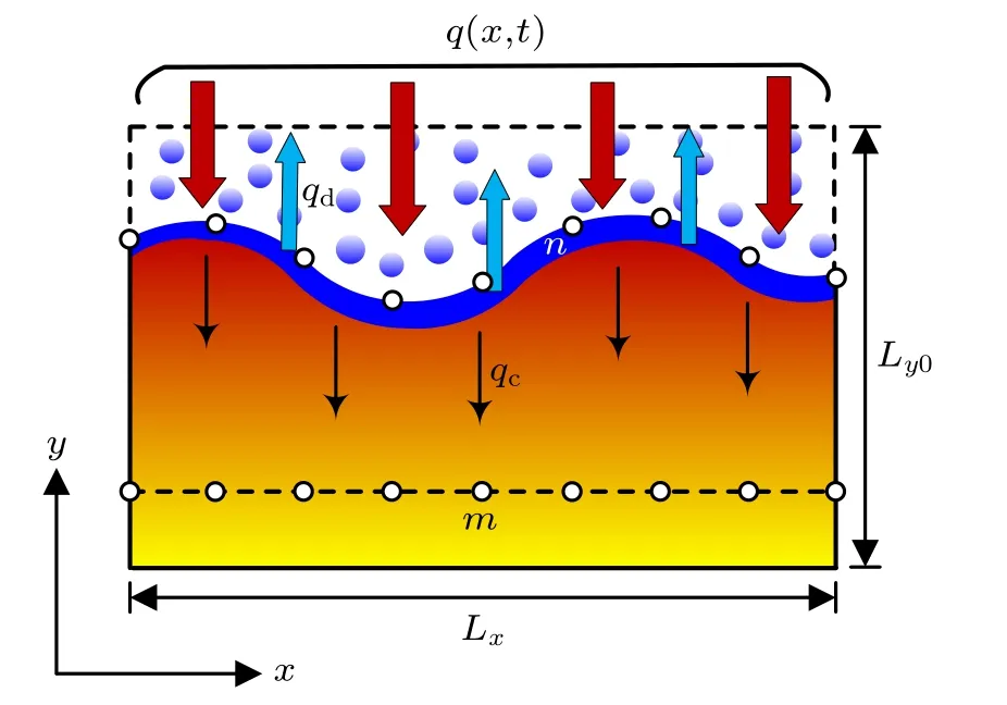
Fig.1. 2D ablation heat transfer system.

The transient temperature field T(x,y,t) of the ablation material is described by the following equation:

with the initial condition

and boundary conditions

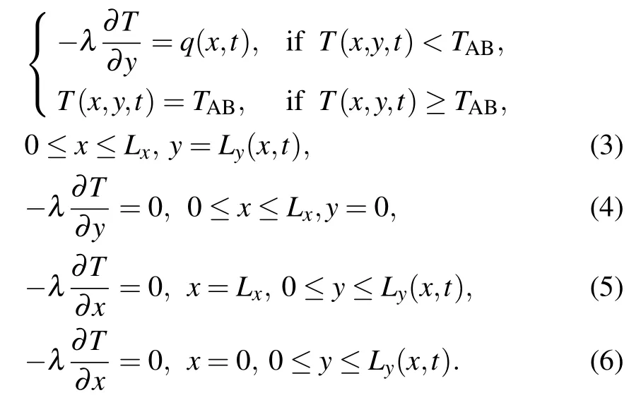
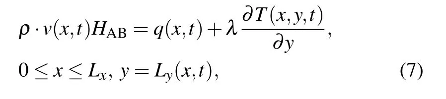
Energy balance equation of the ablated boundary is where a,λ,and ρ are respectively the thermal diffusivity,the thermal conductivity,and the density of the ablation material;T0(x,y)is the initial temperature field; Lxand Ly0are respectively the width and the initial thickness of the material;v(x,t)is the ablation velocity; TABand HABare the phase transition temperature and the latent heat of vaporization of the ablation material,respectively.

2.2. Numerical method of ablation heat transfer

In the numerical simulation process,the heat transfer region is discretized by the quadrilateral mesh.The discrete heat transfer region at the initial moment is shown in Fig.2. The solution domain and mesh division need to be adjusted continuously because the ablated boundary Γ1constantly moves in the ablation process.

Fig.2. Initial mesh of material.

For the mesh division of the solution domain, the temperature governing equations are divided by the finite element method.In the whole solution domain,the discrete form of the above governing equations is composed of the discrete equations of all finite elements.For each element e,the matrix form of the discrete equation is as follows:

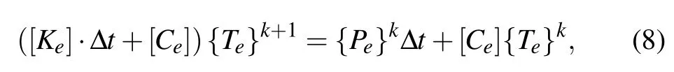
where {Te} is the temperature vector of element; [Ke] is the thermal conductivity matrix of element; [Ce] is the specific heat matrix of element; {Pe} is the heat flux vector of the element. The above compositions of the e-th discrete equation will vary with the geometry of element.

In this paper, the locations of the mesh nodes are online adjusted by the spring analogy method (SAM)[38,39]which can ensure that the topology (number of cells and number of nodes)of the mesh division does not change.

According to the equivalent spring system shown in Fig.3, the static balance is described by the following governing equation:

Fig.3. Spring analogy of variable mesh.

(i) When the i-th node is on the boundary Γ4, the node position is fixed by

(iv)The instantaneous position vectors of the internal grid nodes after deformation are iteratively calculated by the following equation:

with(i=1,2,...,G).In Eqs.(12)and(13), p(p=0,1,2,...)is the number of iterations; I is the number of the nodes on the boundary Γ2and Γ3;G is the number of the internal mesh nodes.

Fig.4. Algorithm flowchart of ablation process simulation.

The numerical simulation of the ablation process is realized by solving the algebraic equations of the heat transfer(i.e.Eq. (8)) and the node position equations (i.e. Eqs. (10)-(13))simultaneously. The above algebraic equations are nonlinear due to the coupling relationship between the heat transfer process and the variable solution domain. When simulating the ablation process,in order to conveniently obtain the solution,the adjustment of the solution domain lags behind the heat transfer process. Setting the number of simulation time steps to be P, the flowchart for numerical simulation procedure of the ablation process is drawn in Fig.4.

2.3. Validation

In order to validate the model and the numerical method,a numerical experiment is carried out. According to Ref.[36],for the system with the width Lx=50 mm and the initial thickness Ly0= 5 mm, thermophysical properties are described by the thermal conductivity λ = 0.2 W/(m·K), the density ρ=2000 kg/m3,the specific heat capacity cp=1000 J/(kg·K),the ablation temperature TAB= 800 K, and the latent heat HAB=2 MJ/kg. Besides, the initial temperature distribution and the total heat flux are respectively T0(x,y)=300 K and q(x,t)=2 MW/m2. The ablation velocity of the simulation is compared with the value of Ref.[36]as shown in Fig.5.

It can be seen that although at the beginning the difference between the two sets of data is larger,with time going by,the simulation result is gradually close to the value of Ref. [36].It is worth noting that the difference at the beginning is due to the switch from conduction simulation to ablation simulation.On a whole,the simulation result is similar to the result in the literature. Therefore,the model and the numerical method are both effective.

Fig.5. Comparison of ablation velocity between simulation and value of Ref.[36].

3. MPIM for estimating ablated boundary heat flux

In the present study, the two-dimensional ablation inverse problem is solved based on the model predictive control theory.[40]

3.1. Objective function

The estimation of the transient heat flux distribution on the ablated boundary can be summarized as a predictive control problem, for which the objective function is established as Eq.(14)to optimize the unknown heat flux matrix Q. For Eq. (14), the first term on the right-hand side describes the relationship between the unknown heat flux matrix and the known measured temperatures,i.e.,the formulation of the 2D ablation inverse problem. Furthermore, considering the illposeness of the 2D ablation inverse problem,the second term is added to improve the stability of the estimation solution.

In Eq.(14):

Y =[Yk, Yk+1, ..., Yk+R−1]T

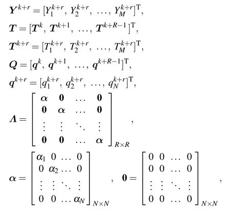
3.2. Predictive model

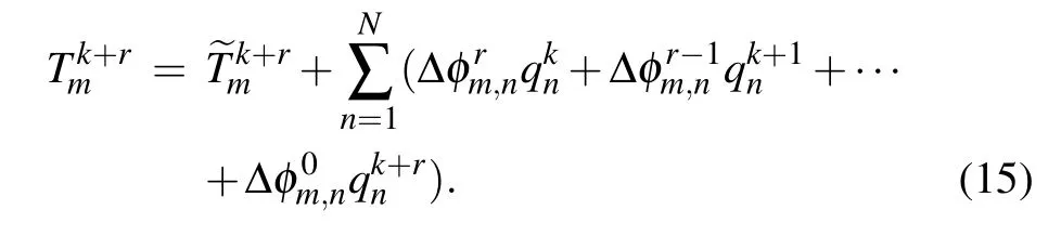
In Eq.(15),

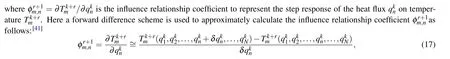
The matrix equation corresponding to Eq. (15) is shown as the following equation:

where

3.3. Rolling optimization of boundary heat flux and ablated boundary reconstruction

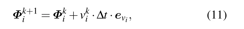
According to Eqs. (14)and(18), the heat flux of the ablated boundary is online estimated by rolling optimization.Then, the estimation value of the heat flux on the ablated boundary is utilized to reconstruct the ablated boundary.

After substituting Eq. (18) into Eq. (14) and ordering dJ(Q)/dQ=0, the optimal heat flux matrix Q in the time domain[tk,tk+R−1]can be obtained to be

where

According to the estimation result of qk, the ablation model Eqs.(1)-(6)and energy balance equation of the ablated boundary are used to obtain the ablation velocity v(x,tk). And, the ablated boundary shape can be reconstructed based on v(x,tk).

4. Numerical experiments and discussion

4.1. Conditions of numerical experiments

Reference[42]shows that the width and the initial thickness of the ablation material are Lx=4 cm and Ly0=2 cm,respectively. The thermal conductivity of the material is taken as λ = 5 W/(m·K), density ρ = 1000 kg/m3, heat capacity cp=1200 J/(kg·K),phase transition temperature TAB=833 K,and latent heat of vaporization HAB=2.326×106J/kg.

Taking M = N = 9, the M temperature measurement points are evenly arranged along the x direction inside the material(y=1.0 cm)and the N estimation points are uniformly set to be on the boundary Γ1.

The transient heat flux distribution loaded to the ablated boundary is assumed as follows:

where ω is the random number obeying the standard normal distribution in the interval [−2.576, 2.576], and σ denotes the standard deviation of the temperature measurement errors.

4.2. Grid independence verification

The time step size is to take Δt =1 s. Different mesh divisions with uniform rectangular unit are chosen to discretize the initial heat transfer domain. When t=75 s,the simulation results of the temperature distribution with different mesh divisions at y=1.0 cm are shown in Fig.6. When the numbers of units are respectively chosen to be 40×40, 60×60, and 80×80,the temperature distributions are similar. Thus,in the subsequent numerical experiment the number of units is taken to be 40×40.

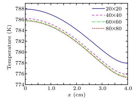
Fig.6. Temperature distribution at y=1.0 cm with different mesh divisions at t=75 s.

The number of uniform rectangular units is taken to be 40×40. The time step sizes are respectively chosen to be Δt =0.5 s, 1.0 s, 2.0 s, and 5.0 s to simulate the temperature evolution with time. The simulation results of time-evolution of temperature with different time step sizes at a measurement point(x=4.0 cm,y=1.0 cm)are shown in Fig.7. According to Fig.7,the time step size is taken to be Δt=1.0 s.

Fig.7. Temperature evolution with time at measurement point(x=4.0 cm,y=1.0 cm)with different time step sizes.

4.3. Estimation and reconstruction results

The number of future time steps is R=8,the standard deviation of temperature measurement errors is σ =0.0 K.Figures 8(a) and 8(b) respectively show the exact heat flux and the estimation result obtained by the MPIM.

Fig.9. (a)The exact value and(b)the reconstruction value of v(x,t).

The exact ablation velocity v(x,t)and the reconstruction result of the ablation velocity v(x,t)are shown in Fig.9.

As shown in Figs. 10 and 11, the estimation results of the boundary heat flux and the reconstruction results of the ablation velocity at x=0 cm and x=4.0 cm are respectively compared with the exact values at the corresponding locations.

Fig.10. Exact and estimation results of(a)boundary heat flux and(b)ablation velocity at x=0 cm.

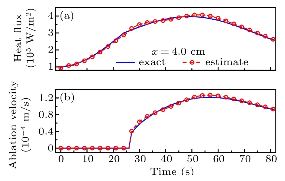
Fig.11. Exact and estimation results of(a)boundary heat flux and(b)ablation velocity at x=4.0 cm.

Figure 12 shows the reconstruction results of the ablated boundary shape and the temperature field of the material at different moments.

Fig.12.Reconstruction results of transient ablated boundary shape and temperature field.

4.4. Effect of measurement errors

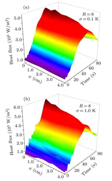
Fig.13. Estimation results of boundary heat flux q(x,t)with σ =0.1 K(a)and σ =1.0 K(b).

Fig.14. Reconstruction results of ablation velocity v(x,t) with σ =0.1 K(a)and σ =1.0 K(b).

The number of future time steps is R = 8. The standard deviation of temperature measurement errors is respectively chosen to be σ =0 K, σ =0.1 K, and σ =1.0 K to investigate the effect of the measurement errors on the result.The estimation results of the boundary heat flux q(x,t) and the reconstruction results of the ablation velocity v(x,t) are shown in Figs.13 and 14,respectively. In addition,the results at x=0 cm and x=4.0 cm are shown in Figs.15 and 16 respectively. The reconstruction results of the ablated boundary shape and the temperature field of the material are shown in Fig.17.

Fig.15. Exact and estimation results of(a)boundary heat flux and(b)ablation velocity at x=0 cm with different values of σ.

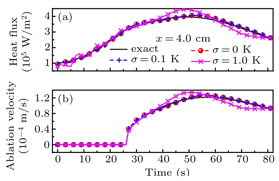
Fig.16. Exact and estimation results of(a)boundary heat flux and(b)ablation velocity at x=4.0 cm with different values of σ.

Fig.17.Reconstruction results of transient ablated boundary shape and temperature field at t=75 s with σ =0.1 K(a)and σ =1.0 K(b).

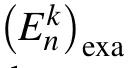
When the standard deviation of the temperature measurement errors σ is taken to be different values, the relative average errors of the results are shown in Table 1. The relative average error is defined by the following equation:

Comparisons between simulation and experiment results in Figs.8-12 and Figs.13-17 indicate that although there exist different temperature measurement errors, the established inverse method can be used to obtain the acceptable estimation results of boundary heat flux and ablation velocity.

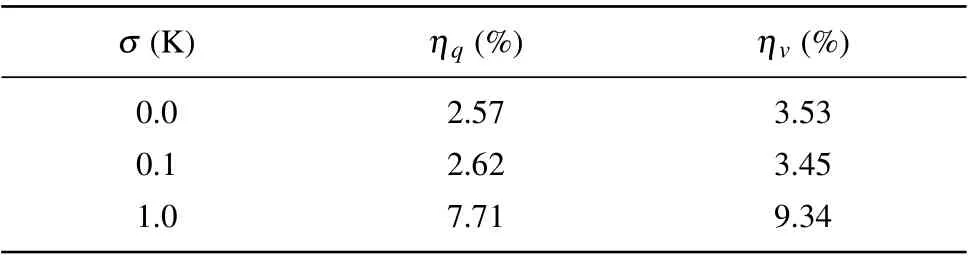
Table 1. Relative average errors of estimation results with different values of σ.

4.5. Effect of the number of future time steps

The standard deviation of temperature measurement errors is σ =0.1 K.The number of future time steps is chosen separately to be R=5, R=8, and R=12 to investigate the effect of the number of future time steps on the results. The estimation results of the boundary heat flux q(x,t)and the reconstruction results of the boundary ablation velocity v(x,t)are shown in Figs.18 and 19,respectively.

Fig.18. Estimation results of boundary heat flux q(x,t)with R=5(a)and R=12(b).

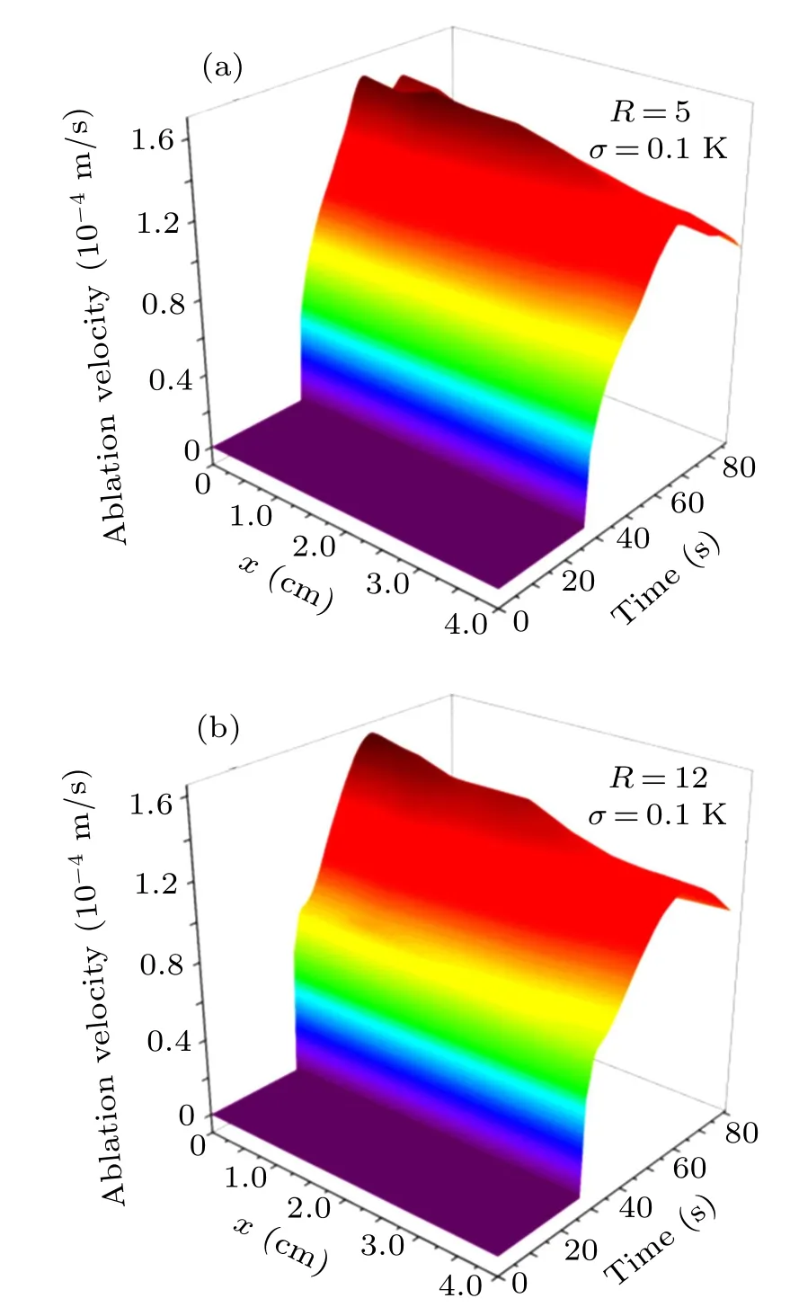
Fig.19.Reconstruction results of ablation velocity v(x,t)with R=5(a)and R=12(b).

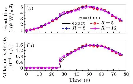
Fig.20. Exact and estimation results of(a)boundary heat flux and(b)ablation velocity at x=0 cm with different values of R.

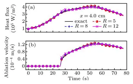
Fig.21. Exact and estimation results of(a)boundary heat flux and(b)ablation velocity at x=4.0 cm with different values of R.

In addition, the results at x=0 cm and x=4.0 cm are shown in Figs.20 and 21 respectively. The reconstruction results of the ablated boundary shape and the temperature field of the material are shown in Fig.22.

Fig.22.Reconstruction results of transient ablated boundary shape and temperature field at t=75 s with R=5(a)and R=12(b).

When the number of the future time steps R is taken to be different values, the relative average errors of the results are shown in Table 2.

Table 2. Relative average errors of results with different values of R.

The simulation experiment results given above(Figs.18-22)illustrate that the inverse method established in this paper has little sensitivity to the number of the future time steps in the scope of above experiments.

4.6. Effect of location of measurement points

The standard deviation of the temperature measurement errors,the number of the future time steps and the number of the measurement points are, respectively, σ =0.1 K, R=8,and M=9. The locations of the measurement points are chosen,respectively,as y=0.6 cm,y=0.8 cm,y=1.0 cm,and y=1.2 cm to investigate the effect of the location of the measurement points on the result. The relative average errors of the results with different locations of the measurement points are shown in Table 3.

Table 3. Relative average errors of results with different locations of measurement points.

It can be known from Table 3 that the closer to the bottom of the ablation material(the farther away from the boundary heat flux) the measurement points, the worse the results of the boundary heat flux estimation and the ablation velocity reconstruction will be. However, the shorter the distance between the measurement points and the boundary heat flux,the less the effect of the location of the measurement points on the results will be.

4.7. Effect of the number of measurement points

The standard deviation of the temperature measurement errors and the number of the future time steps are,respectively,σ =0.1 K and R=8. The location of the measurement points is at y=1.0 cm. The number of the measurement points is respectively chosen to be M=4,M=6,M=9,and M=12 to investigate the effect of the number of the measurement points on the results. The relative average errors of the results with the different numbers of the measurement points are shown in Table 4.

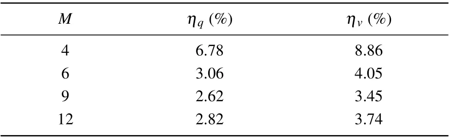
Table 4. Relative average errors of results with different values of M.

According to Table 4, by increasing the number of measurement points,the accuracies of the boundary heat flux estimation results and the ablation velocity reconstruction results are improved. But,the larger the number of the measurement points,the less the improvement extent of the results will be.

5. Conclusions

In this paper, a 2D ablation inverse problem is investigated,and a model predictive inverse method(MPIM)is presented to estimate the unknown heat flux on the ablated boundary of the 2D ablation process. The movement law of the ablated boundary is reconstructed according to the estimation result of the time and space-dependent heat flux.

The MPIM establishes the time-varying predictive model of the temperatures at the measurement points inside the ablation material based on the influence relationship matrix. This method can online estimate the time- and space-dependent heat flux on the ablated boundary by the rolling optimization combining with the predictive model.According to the numerical results,for the presented inverse method,the choice of the number of the future time steps has a marginal effect on the reconstruction results of the boundary conditions,and the acceptable results can be obtained even though the measurement errors of the temperature exist. In addition, the locations and the number of the measurement points can influence the reconstruction results. Appropriately reducing the distance between the measurement points and the boundary heat flux,as well as arranging enough measurement points,can be beneficial to the method presented in this paper.