ON THETA-TYPE FUNCTIONS IN THE FORM (x;q)∞*

Changgui ZHANG

Laboratoire P. Painlev´e (UMR - CNRS 8524), D´epartement de math´ematiques, FST,Universit´e de Lille, Cit´e scientifique, 59655 Villeneuve d’Ascq cedex, France E-mail: changgui.zhang@univ-lille.fr

Abstract As in our previous work [14], a function is said to be of theta-type when its asymptotic behavior near any root of unity is similar to what happened for Jacobi theta functions. It is shown that only four Euler infinite products have this property. That this is the case is obtained by investigating the analyticity obstacle of a Laplace-type integral of the exponential generating function of Bernoulli numbers.

Key words q-series; Mock theta-functions; Stokes phenomenon; continued fractions

1 Introduction

In his last letter to Hardy, Ramanujan wrote that he had discovered very interesting functions that he called mock ϑ-functions. As was said in Watson’s L.M.S.presidential address[10],the first three pages, where Ramanujan explained what he meant by “mock ϑ-functions”, are very obscure. Therefore, Watson quoted the following comment of Hardy:

A mock ϑ-function is a function defined by a q-series convergent when|q|＜1,for which we can calculate asymptotic formulae, when q tends to a “rational point” eof the unit circle,of the same degree of precision as those furnished for the ordinary ϑ-functions by the theory of linear transformation.

In our previous work [14], we proposed definitions of what we call theta-type, false thetatype and mock theta-type functions, following directly from the above-mentioned comment of Hardy. The main goal of this paper is to determine the possible values of x for which the Euler q-exponential function (x;q)is of theta-type, where

1.1 Statement of Main Theorem

The above-named variable qmay be considered as the modular variable with respect to the root ζ. By considering the respective modular formulae,one can easily see that the ordinary ϑ-functions, as well as the famous Dedekind η-function, satisfy the condition in (1.2) for any root of unity ζ.

Let U denote the set of the roots of unity. One remembers that η(τ)=q(q;q), where q =e(τ). Thus, one can observe that (q;q)∈Tfor any ζ ∈U. Furthermore, an elementary calculation shows that the following identities hold:

Theorem 1.2 (Main theorem) Let (x,β)∈C×R be such that |x|=1 and β /=0, and consider x=xq. Then, the following conditions are equivalent:

(1) one has (x;q)∈T, with ζ =1=e(0);

(2) there exists a root of unity ζ =e=e(r) such that (x;q)∈T;

1.2 Some Ideas for the Proof of Main Theorem

If one takes the principal branch of the logarithm for both members of the above equation, one can observe the following fact:

Remark 1.3 (Asymptotic form of the theta-type functions) Given ζ ∈U and f(q)∈T,there exists a quadruplet (υ,c,c,c)∈Q×(iR)×C×(iR) such that

A modular-like formula has been found for (x;q)in [13, Th. 3.2] and [15, Th. 2.9], by means of one certain perturbed factor named P(z,τ), where x = e(z) and q = e(τ). Thus, it suffices to understand the analyticity obstacle of P(α+β τ,τ) around each given rational point τ =r ∈Q ∩[0,1). We shall obtain the condition for this function to be analytically continued at τ =0 by a Stokes analysis, with the help of the Ramis-Sibuya theorem [6, 8]. This analysis will be generalized for every r ∈Q ∩(0,1)by means of a series of transformations associated to the continued fraction of r; transformations often used in the classical theory of the modular functions.

1.3 Plan for the Paper

The rest of the paper is divided into three sections. In Section 2, we define a family of integrals involving the exponential generating function associated with the Bernoulli numbers.These integrals can be seen as being of Laplace type, and they will be used for stating an equivalent version of the above-mentioned result on (x;q); see Theorems 2.1 and 2.4.

Section 3 is essentially devoted to the part ζ =1 of Theorem 1.5;see Theorem 3.1. By means of Theorems 2.1 and 2.4, we will see that the fact that a Euler q-exponential function, modulo some exponentially small term,can be analytically continued at τ =0 and may be interpreted as one problem of the analytic continuation inside the theory of the Gevrey asymptotic expansions;see Theorem 3.8 and the proof of Theorem 1.5 given in Subsection 3.3.

Section 4 aims to obtain Theorem 1.5 for an arbitrary root ζ of unity; see Theorem 4.1.Lemma 4.8 will play a key role, especially in terms of permitting us to make use of both continued fractions and modular transforms. Finally, a complete scheme for proving our main result, Theorem 1.2, will be outlined at the end of the paper.

2 A Laplace-type Integral Involving Bernoulli Exponential Generating Function

In Subsection 2.1, we will introduce a family of Laplace-like integrals denoted as b, involving the exponential generating function of Bernoulli numbers. It will be shown that the term((z-1)/τ|-1/τ)in the right-hand side of (2.1)can be obtained from comparing these integrals in different directions; see Theorem 2.4. One will also see that the same integrals are closely linked to the function P(z,τ) used in Theorem 2.1, and an equivalent version of this theorem will come from this comparison; see Theorem 2.8 in Subsection 2.2.

2.1 Bernoulli Integrals

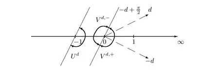
Figure 1 Half-planes Ud, V d,- and V d,+

Proof This follows from [2, p. 36, (21.1)].□

By (2.11), one finds that ((-1,∞)×(CR))⊂W∩W. In what follows, we will write CR=H ∪H, where H=-H={τ ∈C:ℑτ ＜0}.

Theorem 2.4 Let (z,τ)∈W∩W. The following assertions hold:

Figure 2 τ belongs to the common domain V d1,+∩V d2,- while the directions d1 and d2 are separated by the half-line ℓτ

Figure 3 The half-plane Zτ contains both the point τ and the segment (-1,∞)

2.2 Functions related with Bernoulli Integrals

3 Conditions for a Euler q-exponential Function to be of Theta-type at One

We shall make use of the Gevrey asymptotic expansions for understanding the analytic obstacle at τ = 0 of the above-mentioned functions B and P. This is linked to the so-called Stokes’ phenomenon. One tool to treat this problem may be Ramis-Sibuya Theorem, which will be briefly explained in Subsection 3.1 in what follows.

3.1 Ramis-Sibuya’s Theorem on Gevrey Asymptotic Expansions

As a typical example, the Borel-sum function of a given divergent series,if it exists,admits this series as a Gevrey asymptotic expansion. A Gevrey type asymptotic expansion is also called an exponential asymptotic expansion, due to the following fact:

Remark 3.2 ([6, p. 175, Th. 1.2.4.1 1)]) A function f admits the identically null series as a Gevrey asymptotic expansion at 0 in V if and only if f is exponentially small there,which means that, for all proper sub-sectors U in V, there exists C ＞0 and κ ＞0 such that, for all x ∈U, |f(x)|≤C e.

In what follows,we will denote by A(V)the space of all functions that are exponentially small in V as indicated in Remark 3.2. More generally, when V = V(I;R), we will say that f ∈A(V) when f is exponentially small as x →xin V.

Theorem 3.3 ([6,p. 176,Th. 1.3.2.1]) Let V,··· ,V, Vbe a family of open sectors at 0 in C such that V=V, V∩V/=Ø for 1 ≤j ≤m and that the whole union ∪Vcontains a neighborhood of 0 in C. For every j,let fbe a given analytic and bounded function in V. If

On the other hand, if the statement in (3) is true, then both fand fequal to a same analytic and bounded function in the punctuated disc{0 ＜|x|＜R}. By the Riemann removable singularities Theorem, one finds the statements (1) and (2).□

3.2 Asymptotic expansion of Bernoulli integrals

Proposition 3.6 Let (α,β) ∈Rand let I = (-π,π). If α ＞-1, then b(α+β τ,τ) is well-defined and analytic in V(I;R), and is bounded in every proper sub-sector of V(I;R)with R ＞0.

Proof For all τ ∈C, let Dbe the sector containing 0 that is bounded by (-∞,-1]∪[-1,-1- ∞τ), where [-1,-1- ∞τ) denotes the half straight-line starting from -1 to ∞with the direction -τ. By combining (2.8) together with (2.9), one can find that, for all fixed τ ∈C(-∞,0], the function b(z,τ) is defined and analytic for z ∈D.

If α ＞-1, one can easily see that α+β τ belongs to this half-plane Dwhen τ /∈R. This implies that b(α+β τ,τ) is well-defined and analytic in any sector V(I;R).

The boundedness of this function over any proper sub-sector comes from direct estimates done for (2.7).□

In a similar way,one can find that the statement of Proposition 3.6 remains true if b(z,τ)and I are replaced with b(z,τ) and (0,2π), respectively. Thus, one obtains the following:

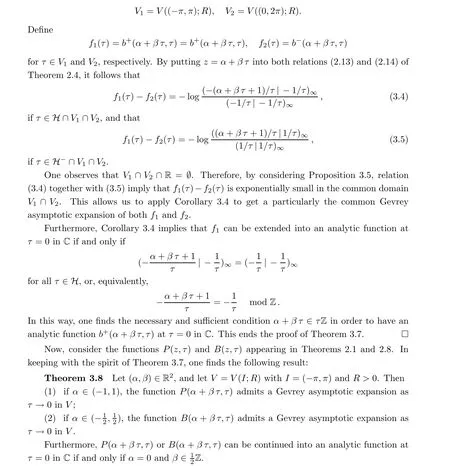
Theorem 3.7 Let (α,β) ∈Rand let b(z,τ) as in Definition 2.2. If α ＞-1, then b(α+β τ,τ) admits a Gevrey asymptotic expansion in any sector V(I;R) with I = (-π,π)and R ＞0.

Moreover,b(α+β τ,τ) can be continued into an analytic function at τ =0 if and only if α=0 and β ∈Z.

Proof Fix R ＞0, and let

3.3 Proof of Theorem 3.1

where ν ∈Q and λ ∈C.

4 Asymptotic Behavior at an Arbitrary Root via Continued Fractions

With regard to an arbitrary root ζ of unity, we shall establish the following result, which,together with Theorem 3.1, will imply Theorem 1.5:

Theorem 4.1 Let r ∈Q ∩(0,1), ζ = e(r) and (α,β) ∈[0,1) × (0,1], and consider f(q)=(α+β τ|τ). Then f ∈Cif and only if α ∈{0,} and β ∈{,1}.

First,one will observe,in§4.1,that the corresponding functions B and P used in Theorems 2.8 and 2.1 are analytic at each non-zero rational point τ =r. This allows us to establish one key lemma, Lemma 4.8, in Subsection 4.2, that permits us to pass an arbitrary rational value r to an other r. By iterating this procedure, one arrives at the case of r = 0, to which case Theorem 3.1 can be applied. This is realized in terms of the continued fractions relative to r and related modular transforms; see Theorem 4.9 in Subsection 4.3. We complete the proofs of Theorems 4.1, 1.5 and 1.2.

4.1 Bernoulli Integral and Associated Functions on a Real Axis

We will discuss the degenerate case τ ∈Rfor the functions b(z,τ), B(z,τ)and P(z,τ).In what follows, we will make use of the notational convention

When ǫ →0,Wbecomes(0,∞)and-W-1 is reduced into C(-∞,-1]. By replacing τ with r in the partial lattice Δgiven by (4.2) for all τ ∈H, we will continue to write Δ= {n+mr : n ∈Z,m ∈Z}. It is easy to see that Δis discrete on the real axis if and only if r is a rational number. In this way, we shall make use of the following remark:

Figure 4 b+(z,τ) is analytic for z ∈(-W∈c-1) and τ ∈W∈

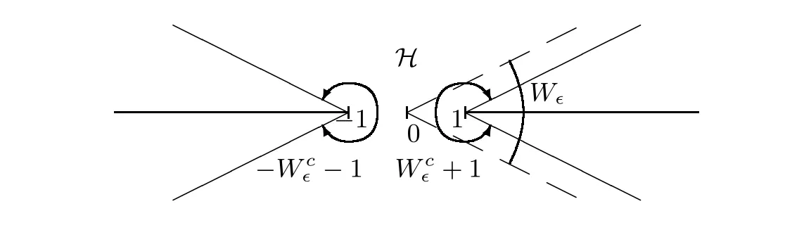
Figure 5 P(z,τ) is analytic for z ∈(-Wc∈-1)∩(Wc∈+1) and τ ∈W∈

Similarly to Remark 4.3, one can observe the following property:

4.2 One Key Lemma

As in the definition of ˘b(z,r) in (4.4), we will let [a] and {a} denote the integral and fractional part, respectively, of any given real a. Given each non-zero real r, consider the

By noticing the relation τ-r= (τ -r)/(rτ), it follows from (4.13) that g(q) ∈Cif and only if ～g(q) ∈C. Thus, we shall use Theorems 2.8 and 2.1 to link f(q) with ～g(q) in the following fashion:

4.3 Continued Fractions and Modular Transforms

Theorem 4.9 Let (ν,r), τand z(τ) be given as in (4.18) and (4.19), with (α,β) ∈[0,1)×(0,1]. Let ζ=e(r) and q=e(τ) for j from 0 to ν. Consider

Proof of Theorem 4.1 This follows directly from Theorem 4.9.□

Proof of Theorem 1.5 In view of Theorems 3.1 and 4.1,it suffices to notice that,given ζ ∈U, one has (xq;q)∈Cif and only if the same holds by replacing β with β+1. This last equivalence can be deduced from the relation (xq;q)= (1-xq)(xq;q)and the fact that (1-xq)∈C, for C{0} constitutes a multiplicative group.□

Proof of Theorem 1.2 By taking into account Remark 1.1 and Theorem 1.5,one needs only to observe that, for any positive integer n ∈Zand any root ζ ∈U, any finite product of the form (xq;q)does not belong to T, although the same function belongs to the larger class C.□

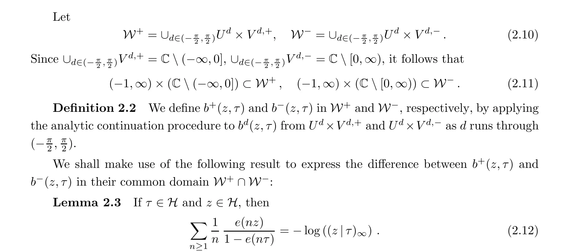
Addendum After having finished a first version of our paper, we learned that the interesting work [4] is closely related to the present paper. Indeed, let α ＞0 and μ ∈[0,1) be as in[4, Theorem 1]. By combining [4, (3.2) & (3.3)] together with (1.2) and (1.4), one can observe the following result:

Remark 4.10 One has(e(μ)q;q)∈Tonly if the following conditions are satisfied for all integers k ≥2: