Geometry on the Wasserstein space over a compact Riemannian manifold

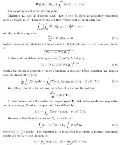
The introduction of tangent spaces of P(M) goes back to the early work [1], as well as in[2]. A more rigorous treatment was given in [3]. In differential geometry, for a smooth curve{c(t); t ∈[0,1]} on a manifold M, the derivative c(t) with respect to the time t is in the tangent space : c(t) ∈TM. A classical result says that for an absolutely continuous curve{c(t); t ∈[0,1]} on M, the derivative c(t) ∈TM exists for almost all t ∈[0,1]. Following[3],we say that a curve{c(t); t ∈[0,1]}on P(M) is absolutely continuous in Lif there exists k ∈L([0,1]) such that

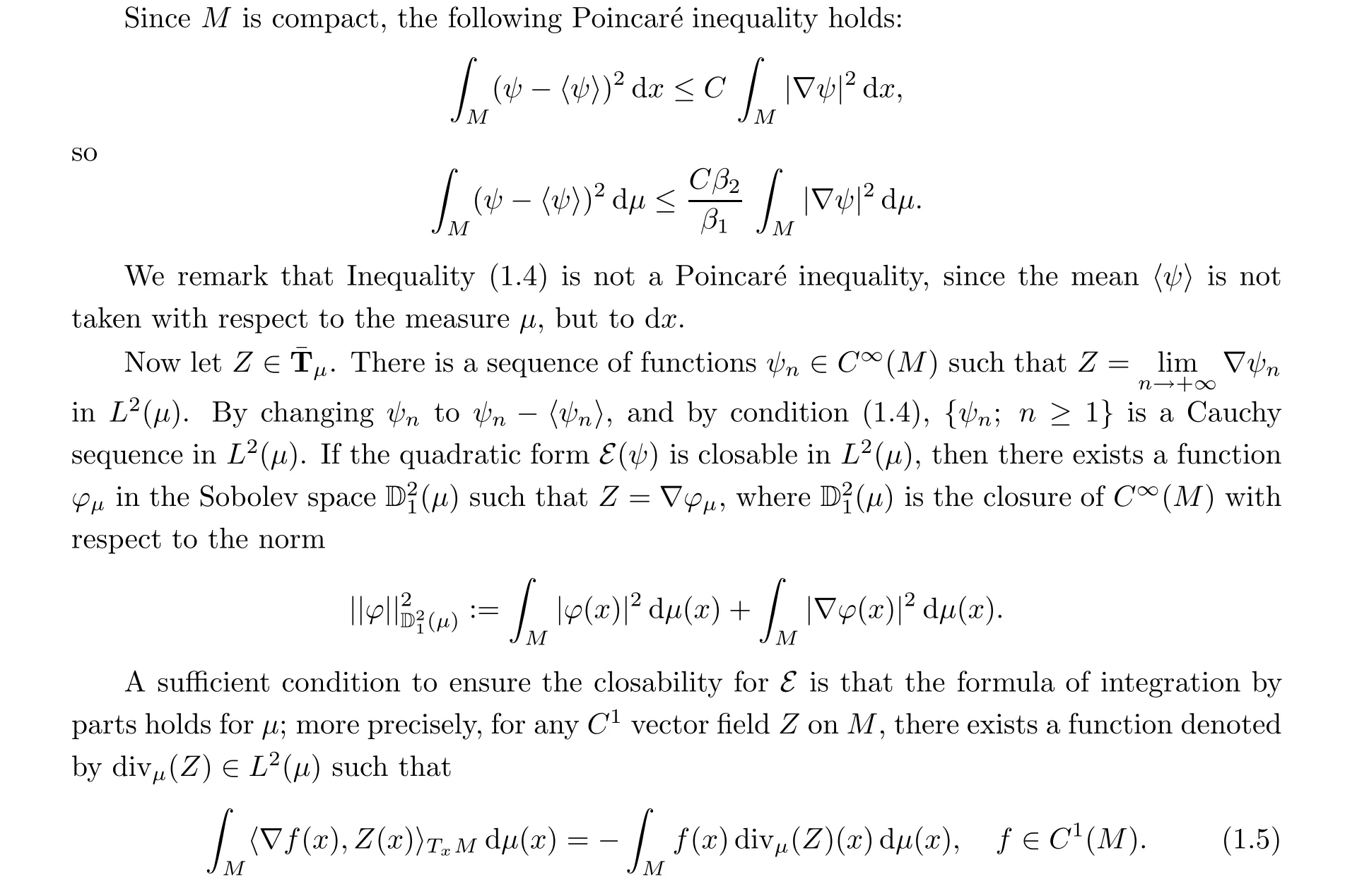
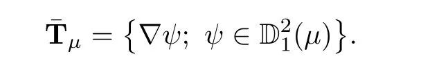
Definition 1.2 We say that a probability measure μ has divergence if div(Z) ∈L(μ)exists. We will use the notation P(M)to denote the set of probability measures on M having strictly positive continuous density and satisfying conditions (1.5).

For example, μ ∈P(M) if dμ(x)=ρ(x)dx for some strictly positive continuous density ρ ∈D(dx).

Proposition 1.3 For a measure μ ∈P(M), we have

Note that this result is not new; see for example [4, 5]. Here we indicate the conditions necessary to yield this result.

The inconvenient thing for (1.3) is the existence of a derivative for almost all t ∈[0,1]. In what follows, we will present two typical classes of absolutely continuous curves in P(M).

1.1 Constant vector fields on P2(M)

For any gradient vector field ∇ψ on M with ψ ∈C(M),consider the ordinary differential equation (ODE)

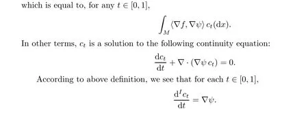
This is why we call ∇ψ a constant vector field on P(M). In order to make clearly the different roles played by ∇ψ, we will use notation Vwhen it is seen as a constant vector field on P(M).

Remark 1.4 In Section 3 below, we will compute Lie brackets of two constant vector fields on P(M) without explicitly using the existence of density of measure; the Lie bracket of two constant vector fields is NOT a constant vector field.

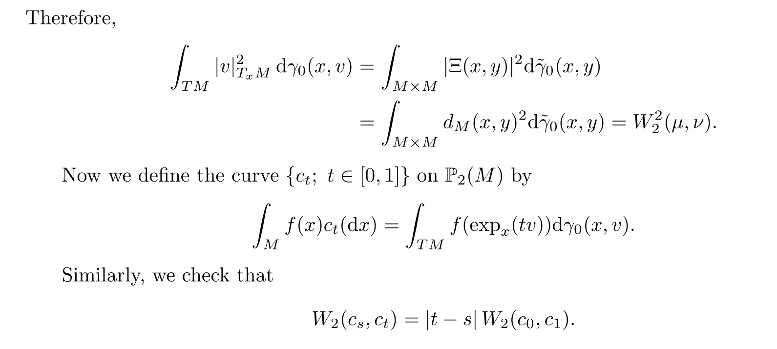
1.2 Geodesics with constant speed

We remark that {∇ψ,t ∈]0,1[} satisfies, heuristically, the equation of the Riemannian geodesic obtained in [6] or that which is heuristically obtained in [1], in which the authors showed that the convexity of the entropy functional along these geodesics is equivalent to Bakry-Emery’s curvature condition [7] (see also [4, 8-10]).

In the case of the Riemannian manifold M, things are a bit complicated. We follow the exposition of [11]. Let TM be the tangent bundle of M and let π : TM →M be the natural projection. For each μ ∈P(M), we consider the set

The organization of this paper is as follows: in Section 2, we consider ordinary equations on P(M), a Cauchy-Peano’s type theorem is established, and the Mckean-Vlasov equation is involved. In Section 3, we emphasize that the suitable class of probability measures for developing the differential geometry is one having divergence and strictly positive density with certain regularity. The Levi-Civita connection is introduced and the formula for the covariant derivative of a general but smooth enough vector field is obtained. In Section 4, we give the precise result on the derivability of the Wasserstein distance on P(M), which enable us, in Section 5 to obtain the extension of a vector field along a quite good curve on P(M), as in differentiable geometry; the parallel translation along such a good curve on P(M) is naturally and rigorously introduced. The existence for parallel translations is established for a curve whose intrinsic derivative gives rise to a good enough vector field on P(M).

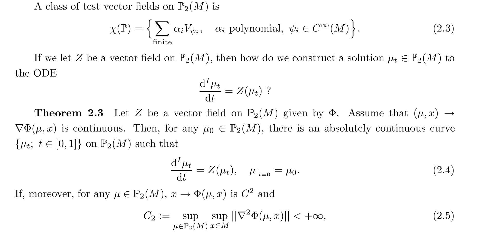
2 Ordinary Differential Equations on P2(M)

Note that the family {F, φ ∈C(M)} separates the point of P(M). By the Stone-Weierstrauss theorem, the space of polynomials is dense in the space of continuous functions on P(M).

Remark 2.1 If the gradient ∇ψ is replaced by a general C-vector field on M,the above definition is also well-established;in fact this was done in the early work[12]in another context for other applications. The links among different types of derivatives were recently characterized in [13].

Convention of notations We will use ∇to denote the gradient operator on the base space M, and ¯∇to denote the gradient operator on the Wasserstein space (P(M),W). For example, if (μ,x) →Φ(μ,x) is a function on P(M)×M, then ∇Φ(μ,x) is the gradient with respect to x, while ¯∇Φ(μ,x) is the gradient with respect to μ.

Definition 2.2 We will say that Z is a vector field on P(M) if there exists a Borel map Φ:P(M)×M →R such that, for any μ ∈P(M), x →Φ(μ,x) is Cand Z(μ)=V.

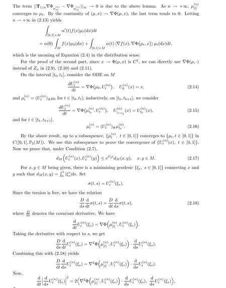
then there is a flow of continuous maps (t,x) →U(x) on M that forms a solution to the following Mckean-Vlasov equation:

By the Ascoli theorem, up to a subsequence, μconverges in C([0,1],P(M)) to a continuous curve {μ; t ∈[0,1]} such that W(μ,μ)≤2C(t-s).

For proving that {μ; t ∈[0,1]} is a solution to ODE (2.4), we need the following preparation:

Remark 2.5 Comparing this to [14], as well to [15], we do not suppose the Lipschitz continuity with respect to μ; accordingly, we have no uniqueness of solutions of (2.6).

Remark 2.6 Many interesting PDE can be interpreted as gradient flows on the Wasserstein space P(M)(see[3,16-18]). The interpolation between geodesic flows and gradient flows were realized using Langevin’s deformation in [4, 5].

3 Levi-Civita Connection on P2(M)

In this section,we will revisit the paper by Lott[6];we will try to reformulate the conditions given there as weakly as possible, and also to expose some of them in an intrinsic way,avoiding the use of density. In order to obtain a good picture of the geometry of P(M), the suitable class of probability measures should be the class P(M)of probability measures on M having divergence (see Definition 1.2).

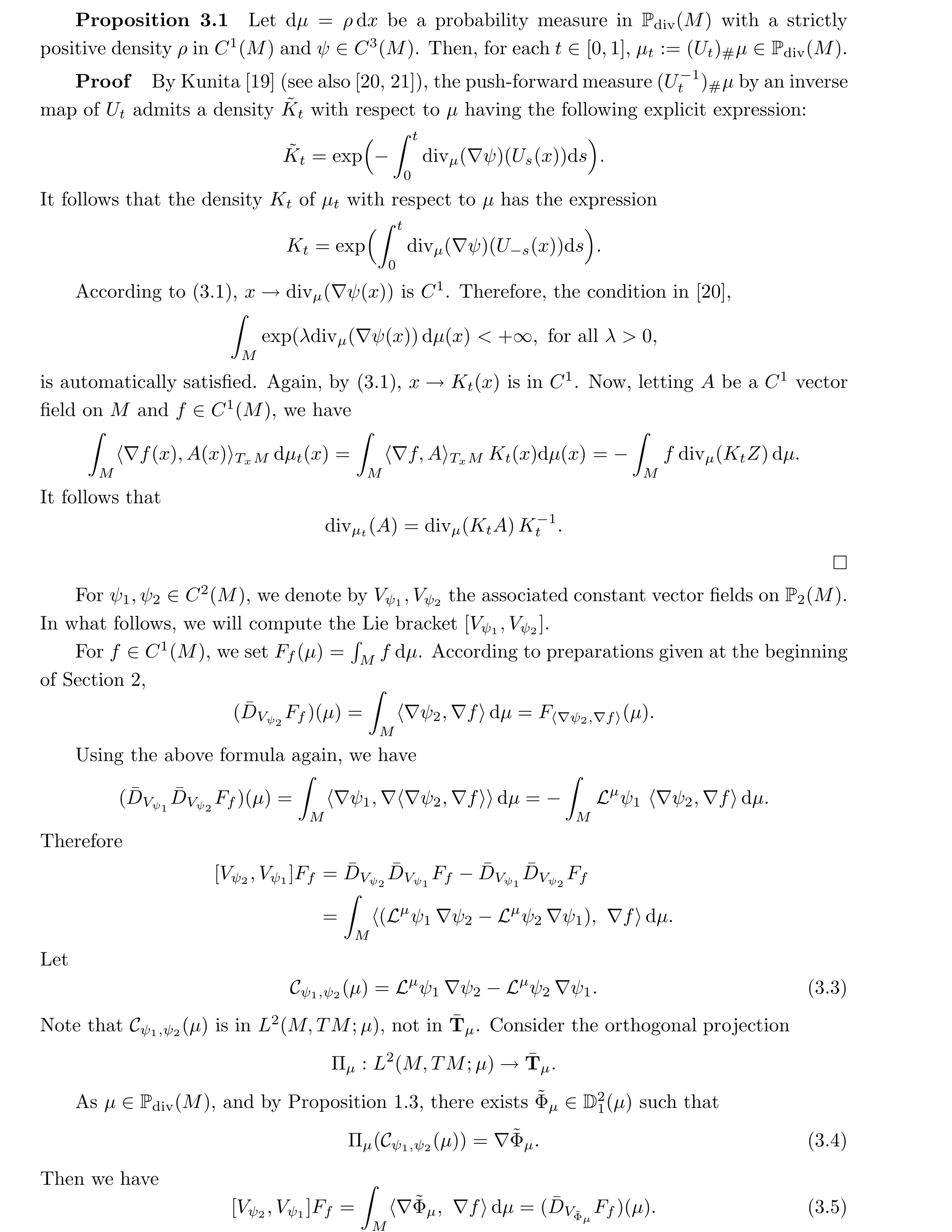
The above equality can be extended to the class of polynomials on P(M) ; that is to say

We emphasize that the Lie bracket of two constant vector fields is no longer a constant vector field.

Proposition 3.2 Letting ψ,ψ∈C(M), for dμ=ρ dx with ρ ＞0 and ρ ∈C(M), the function ～Φobtained in (3.4) has the following expression:

It follows that ～Φhas the expression (3.7).□

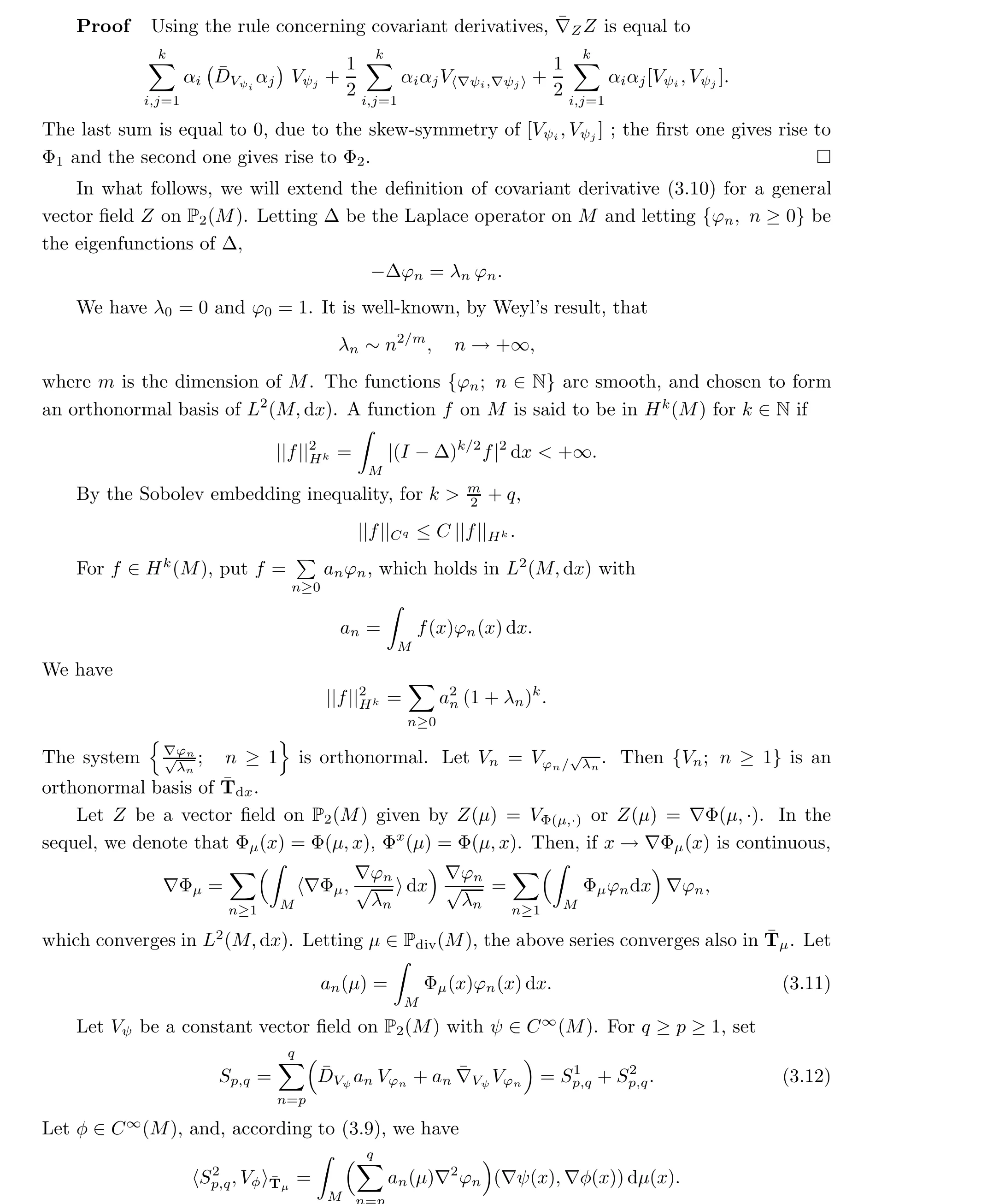
Letting q →+∞yields the result.□

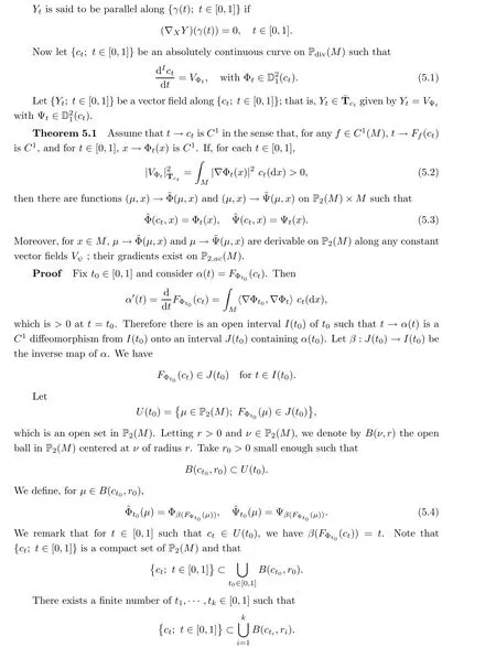
4 Derivability of the Square of the Wasserstein Distance

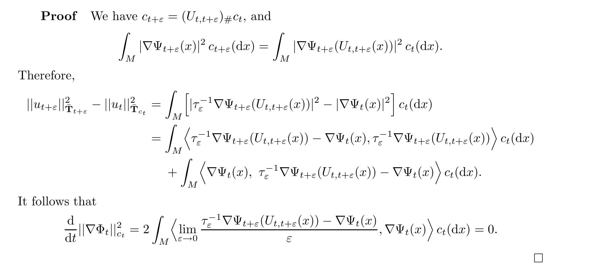
Proof See [25], page 10.□

from which we get (4.2). The proof is complete.□

5 Parallel Translations

Before introducing parallel translations on the space P(M), let us give a brief review on the definition of parallel translations on the manifold M, endowed with an affine connection.Let {γ(t); t ∈[0,1]} be a smooth curve on M, and {Y; t ∈[0,1]} be a family of vector fields along γ: Y∈TM. Then there exist vector fields X and Y on M such that

Then (5.8) follows from (3.13).□

In what follows, we will slightly relax the conditions in Proposition 5.5. We return to the situation in Theorem 5.1. Let {c;t ∈[0,1]} be an absolutely continuous curve in P(M)satisfying the conditions in Theorem 5.1 and set

Under the assumption of the uniqueness of the solution to (5.14), we get that c= μfor t ∈[0,1]. Now, by the same arguments as those in the proof of Propositions 5.5 and 5.6, we obtain the result.□

The result follows.□

Theorem 5.10 Letting Z be a vector field on P(M) satisfying the Lipschitz condition(5.15), the ODE

Acknowledgements This work was prepared as part of a joint PhD program between the School of Mathematical Sciences, University of Chinese Academy of Sciences (Beijing,China),and the Institute of Mathematics of Burgundy,University of Burgundy(Dijon,France).The first named author is grateful to the hospitality of these two institutions and the financial support of China Scholarship Council is particularly acknowledged. The two authors would also like to thank the referees for their careful reading of the paper and their useful suggestions.