Estimation of the Reflection of Internal Tides on a Slope

WANG Shuya, CAO Anzhou, CHEN Xu, LI Qiang, SONG Jinbao, and MENG Jing

Estimation of the Reflection of Internal Tides on a Slope

WANG Shuya1), CAO Anzhou2), *, CHEN Xu1), LI Qiang3), SONG Jinbao2), and MENG Jing4)

1) Key Laboratory of Physical Oceanography, Qingdao Collaborative Innovation Center of Marine Science and Technology (CIMST), Ocean University of China, and Qingdao National Laboratory for Marine Science and Technology, Qingdao 266100, China 2) Ocean College, Zhejiang University, Zhoushan 316021, China 3) Graduate School at Shenzhen, Tsinghua University, Shenzhen 518055, China 4) College of Oceanic and Atmospheric Sciences, Ocean University of China, Qingdao 266100, China

Reflection occurs when internal tides impact on a steep continental slope. Separating reflected internal tide signals from incident ones is crucial to develop the parameterization of internal tide-driven turbulent mixing on the continental slopes. In this study, the performances of three different methods for estimating internal tide reflections are examined by using two different cases. The Hilbert transform-based method is found to be more suitable than two other methods for both cases considered in this study. The two other methods are effective for westward-propagating mode-1 internal tides impacting a slope, but inappropriate in the case where internal tides radiate from a Gaussian ridge impact the slope because of their inaccurate estimation of incident internal tides in the latter case. Such inaccurate estimation further influences the extraction of reflected signals and calculation of the reflected and cross term of energy fluxes. In addition, it should be noted that, due to the use of filtering, the method based on Hilbert transform may result in slight bias when assessing the incident and reflected signals near topographic features.

internal tide; reflection; continental slope; Hilbert transform; energy flux; filtering

1 Introduction

Internal tides are a ubiquitous motion in stratified oceans, which are generated by barotropic tidal currents flowing over rough topographies, such as mid-ocean ridges, submarine seamounts, continental slopes and shelves (Bell, 1975; Baines, 1982; Chen, 2017; Wang, 2018b; Nie, 2019). As an important intermediate step of the oceanic energy cascade (Rudnick, 2003; Garrett, 2003a, 2003b), internal tides play crucial roles in a number of dynamic processes in the ocean, especially turbulent mixing (Munk and Wunsch, 1998; Carter, 2012).In the open ocean, internal tides can travel more than 1000km from their generation sites (, Ray and Mitchum, 1996; Alford, 2003; Rainville and Pinkel, 2006; Zhao, 2010, 2016; Xu, 2016; Zhao, 2017; Wang, 2018c) before arriving at remote continental slopes (Nash, 2004; Kelly and Nash, 2010; Martini, 2011, 2013).

When internal tides impact a continental slope after long-range propagation, transmission, reflection and dissipation occur, which depend on the criticality parameter

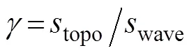
wheretopois the slope of the topography,

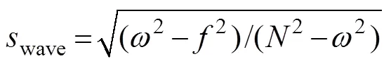
is the slope of the internal tide characteristics with,andrepresenting buoyancy, tidal and Coriolis frequencies, respectively. For a subcritical slope (<1), most of internal tide energy can transmit on it. However, for a supercritical slope (>1), a large fraction of internal tide energy is reflected. In these two situations, the linear theory is generally satisfied. However, when internal tides shoal on a critical slope with=1, the linear theory cannot hold, and nonlinear effects should be considered, which contribute to the breaking and dissipation of internal tides (Dauxois, 2004) hence enhancing turbulent mixing on the slope (Legg, 2014). In addition, scattering of internal tides also occurs when they impact the slope (, Muller and Liu, 2000; Klymak, 2011; Kelly, 2013a, 2013b; Mathur, 2014; Wang, 2019).

In the real oceans, a considerable amount of energy of low-mode semidiurnal internal tides is reflected by continental slopes (Kelly, 2013b). Therefore, understanding the reflection of internal tides on the slope is necessary, and how to separate incident and reflected signals of the internal tides must be solved. Parameterization of internal tide-driven turbulent mixing on continental slopes is also crucial (MacKinnon, 2017) since the incident signals drive local turbulence (Klymak, 2016, hereafter referred as K16). Recent numerical simulations have focused on the reflection of internal tides on continental slopes. For example, Hall(2013, hereafter referred as H13) investigated the influence of depth-varying stratification on the reflection of internal tides and found that the depth of pycnocline almost has no influence on the reflection of incident mode-1 internal tides. Following H13, Wang(2018a) showed that the existence of an abrupt junction point on the shelf break contributes to the reflection of higher modes. In addition to these idealized cases, K16 explored the reflection of mode-1 M2internal tides occurring on the Tasman Slope and revealed that 76% of the incident energy is reflected by supercritical slopes.

Although both H13 and K16 investigated the reflection of internal tides, different methods were used to separate the incident and reflected signals from the total fields of internal tides. In addition, Mercier(2008, hereafter referred as M08) used the Hilbert transform to design an algorithm to discriminate internal waves propagating in different directions. This approach is different from those used by H13 and K16 and has been widely used in laboratory experiments (, Peacock, 2009; Mercier, 2013; Sutherland, 2015; Ghaemsaidi, 2016). Given this background, we are motivated to compare these three methods and evaluate their applicability in different cases of internal tide reflection. First, how the three methods separate reflected signals and two relevant numerical models are introduced. Then, the performances of the three methods in the estimation of reflected internal tides on a slope in two cases are shown. Finally, similarities and differences among the results of the three methods are discussed.

2 Methodology

2.1 Three Methods to Separate Incident and Reflected Internal Tides

2.1.1 H13 method

Part of the energy of internal tides impacting a steep supercritical slope will be reflected. Therefore, the wave field simultaneously includes both the incident and reflected internal tides. To separate the reflected internal tides from incident ones, H13 assumed that the total energy flux equals to the sum of the incident and reflected energy fluxes,,

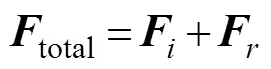
Here the energy fluxis calculated as

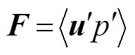
whereis the baroclinic current,is the pressure perturbation, and < > denotes the average over a tidal period (, Kunze., 2002; Nash, 2005). In H13,totalis calculated from the simulated results of internal tides shoaling on the slope andis calculated from the simulated results of a control run in which the slope is artificially removed. Thereafter,is obtained by subtractingfromtotal.

2.1.2 K16 method

Unlike the H13 method, the K16 method assumes that baroclinic current and pressure perturbation can be divided into incident and reflected signals,,

Therefore,

wherecis the cross term of the energy flux; this parameter represents the major difference between this me- thod and H13. Moreover, it should be noted that in this method,andare obtained from the simulated results of the control run, the same as the H13 method. Therefore, the incident energy fluxes calculated by using the H13 and K16 methods are identical.

2.1.3 M08 method

M08 put forward a method to discriminate internal waves propagating in different directions with a given frequency on the basis of the Hilbert transform as well as filtering, Fourier transform, and its inverse transform. M08 also showed detailed procedures on how these internal waves are extracted in the one-dimensional () and two-dimensional (-) cases and applied the method to investigate the reflection and diffraction of internal waves on a slope. In the present study, the M08 method is used to distinguish the incident (and) and reflected (and) signals of internal tides from the total fields of baroclinic current and pressure perturbation. Thereafter, the incident and reflected energy fluxes as well as the cross term (,and) are calculated by using Eq. (6). In this method, the simulated results of the control run, which is essential in both the H13 and K16 methods, are not needed.

2.2 The MITgcm and Its Configuration

The Massachusetts Institute of Technology general circulation model (MITgcm, Marshall, 1997), which solves non-hydrostatic equations under the Boussinesq approximation, is applied to this study. The model is run in hydrostatic mode, because non-hydrostatic process (, the breaking of internal tides) are beyond the scope of this study. The domain is in a two-dimensional (-) plane which is 1200km long and 3000m deep. Both the horizontal and vertical resolutions are uniform,,=1km and=15m. The horizontal viscosityνand vertical viscosityνare set to 10−2m2s−1and 10−3m2s−1, respectively, which are the same as those in H13 and Wang(2018a). The diffusivity is set to zero so that the stratification cannot be eroded in the absence of motion (Legg and Adcroft, 2003). Uniform stratification is considered with the buoyancy frequency=2.8×10−3s−1. The Coriolis frequencyis set to 5.27×10−5s−1, corresponding to a latitude of 21˚N. The free-slip boundary condition is applied to the bottom boundary. Sponge layers are added to the east and west open boundaries to avoid boundary reflection.

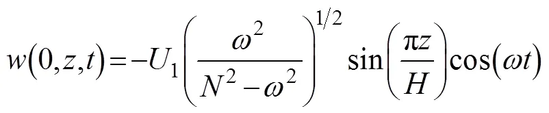
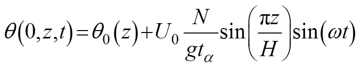
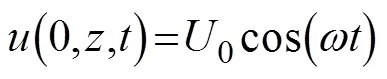
In this study, two cases are examined. Because the diurnal internal tides have lower frequencies (large criticality parameter according to Eq. (2)) than the semi-diurnal internal tides, the former are more easily reflected by continental slopes than the latter (Wu, 2013). Therefore, the K1internal tide is considered in this study. In case 1, westward propagating mode-1 K1internal tides impact a slope (Fig.1, blue folded line). Therefore, the model is forced by the oscillating baroclinic current and temperature anomaly, consistent with the mode-1 K1internal tides at the east open boundary (Legg and Adcroft, 2003, H13; Wang, 2018b):

where1andare the forcing amplitude and frequency of the mode-1 K1internal tides, respectively,is the depth of the domain,0() is the initial profile of the potential temperature,is the acceleration due to gravity, andtis the thermal expansion coefficient. In case 1, the forcing amplitudeof incident K1internal tides is1=2cms−1. In the control run of this case, the slope is removed and the flat seafloor (Fig.1, black line) is considered. The Orlanski radiation boundary condition is applied to the west open boundary to allow the incident waves to propagate out of the domain. In case 2, the incident K1internal tides on the slope are generated from a Gaussian ridge (Fig.1, red curve). In this case, the model is forced by oscillating K1barotropic currents at the east open boundary:

where U0 is the amplitude of the K1 barotropic tidal current and set to 2cms−1. The generation of internal tides from the Gaussian ridge with barotropic tidal forcing at the east open boundary is simulated as the control run. No forcing is added to the west open boundary and sponge layers are applied to the two open boundaries to avoid the boundary reflection of internal waves. In both cases and their corresponding control runs, the model is operated for 10 days and the simulated results are output every one hour. Results in the last tidal period are used in the following analysis.

2.3 The Coupling Equations for Linear Tides Model and Its Configuration

The coupling equations for linear tides model (CELT), which was developed by Kelly(2013a), can determine the independent modal solutions to Laplace’s tidal equations over a stepwise topography in one horizontal dimension. It is a useful tool to investigate the generation, propagation, transmission, and reflection of internal tides in the two-dimensional (-) domain. Unlike the MITgcm, the CELT is a linear model. In this study, the CELT is adopted to simulate the generation of K1internal tides upon the Gaussian ridge (Fig.1, red curve) and reflection on the slope (Fig.1, black line). In other words, the CELT isused to valuate case 2 described above. Because the CELT considers waves traveling to the east and west when it solves Laplace’s tidal equations (Kelly, 2013a), we can obtain the total fields of baroclinic current and pressure perturbation as well as their eastward- and westward-propagating components. The accuracy of the M08 method can then be validated on the basis of these results.

The CELT configuration features horizontal and vertical resolutions of 1.5km and 6m, respectively. In total, 15 vertical modes are taken into account. The viscosity is set to 10−3m2s−1. These settings are different from those applied to the MITgcm, as in Kelly(2013a), since the two models actually employ different governing equations as well as solution methods. The buoyancy and Coriolis frequencies in the CELT are the same as those used in the MITgcm. The CELT only outputs the complex amplitudes of baroclinic current and pressure perturbation; the resulting data are then used to recreate the corresponding time series, which are further analyzed by using the M08 method.

3 Results and Discussion

3.1 Case 1: Reflection of Mode-1 Internal Tides

Fig.2 illustrates the total, incident, reflected and cross term of energy fluxes in case 1 obtained by using the three methods. Because a control run is essential in the H13 and K16 methods but unnecessary in the M08 method, the incident and reflected signals upon the slope extracted by the three methods are not consistent. Moreover, the reflected energy fluxes calculated by the H13 and K16 methods upon the slope (−500km<<−400km) are inaccurate because the topographies are different be-tween case 1 and its control run. Therefore, we only focus on the results obtained from the eastern portion of the slope (>−400km in this case). As shown in Fig.2, the three methods almost give the same pattern of energy fluxes for both incident and reflected internal tides. For the incident internal tides, since no barrier exists along the propagating path, the westward energy flux remains nearly constant during propagation. The energy flux of reflected internal tides reaches a maximal value at the base of the slope (=−400km). With the increase of, the eastward energy flux gradually decreases and reaches nearly zero at approximately=0. These dynamic processes are all well captured by the three methods. However, the M08 method slightly underestimates the incident energy flux and overestimates the reflected energy flux in a small region (−400km<<−350km) because of the use of filtering, which causes some bias in the filtering boundaries. For the region>−350km, the incident and reflected energy fluxes extracted by the M08 method are the same as those extracted by the H13 and K16 methods.

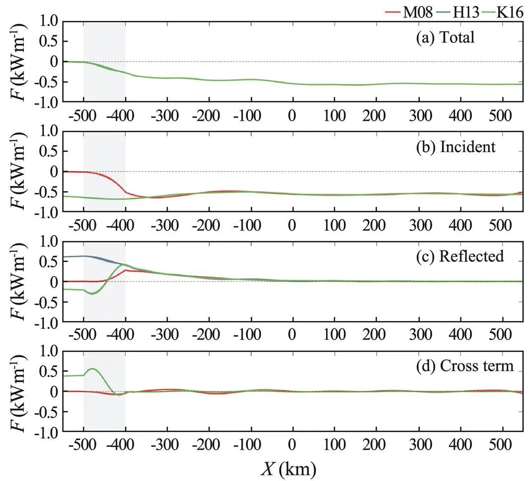
Fig.2 (a) Total, (b) incident, (c) reflected, and (d) cross term of energy fluxes in case 1. Red, blue and green curves denote results obtain by using the M08, H13 and K16 methods, respectively. The total energy fluxes shown in (a) are the same for the three methods and the incident energy fluxes shown in (b) are the same for the H13 and K16 methods. No cross term of the energy flux exists in the H13 method. The blue shadings indicate the location of the slope.

Special attention should be paid to the cross term of the energy flux shown in Fig.2d. As noted by K16, the cross term of the energy flux is not negligible for realistic forcing and causes an interference pattern when internal tides are reflected in the three-dimensional case. However, the cross term of the energy flux is equal to zero in the two-dimensional case in this study. Indeed, these two results are not contradictory. In K16, the cross term of the energy flux is nearly perpendicular to the gradient direction of the slope (Figs.8c and 9c in K16). In other words, the cross term of the energy flux is close to zero along the gradient direction of the slope, which is just the result of the two-dimensional case in this study. The zero cross term of the energy flux in this case also indicates that the H13 and K16 methods are essentially the same when evaluating the two-dimensional (-) reflection of incident internal tides.

In summary, all three methods introduced in Section 2.1 can capture the dynamic processes of incident internal tides reflecting on a slope. Compared with the H13 and K16 methods, however, the M08 method may result in slight bias when assessing the incident and reflected energy fluxes near the slope due to the use of filtering. The H13 and K16 methods are essentially the same for the two-dimensional (-) reflection of incident internal tides, because the cross terms of the energy flux are equal to zero.

3.2 Case 2: Reflection of Internal Tides Radiated from a Gaussian Ridge

In this section, we examine the performances of the three methods when dealing with the slope reflection of the K1internal tides radiated from a Gaussian ridge (Fig.3). Given the existence of the slope and Gaussian ridge, we only focus on the results between them (−400km<<50km in this case). Unlike the results in case 1, the incident and reflected energy fluxes extracted by the three methods in this case show apparent differences. First, for the incident internal tides, the M08 method once again underestimates the westward energy flux compared with the H13 and K16 methods. In addition to the small regions near the slope and Gaussian ridge (−400km<<−350km and −50km<<0km) where the underestimation is caused by the use of filtering, slight underestimation is also found at −350km<<−200km. Second, the cross term of the energy flux calculated by the K16 method is no longer equal to zero at −400km<<50km; instead, it is always positive in this region, corresponding to an eastward pro- pagating signal. By contrast, the cross term calculated by the M08 method is close to zero in this region. Thus, the reflected energy fluxes estimated by the three methods differ significantly. The H13 method leads to the largest estimation of the reflected energy flux and is followed by the M08 method, whereas the K16 method yields the smallest estimation. These results suggest that at least two of the three methods are unsuitable for dealing with the slope reflection of internal tides generated from a ridge. A detailed explanation of these findings is presented in Section 3.4 after we compare the CELT output and results extracted by using the M08 method in Section 3.3.

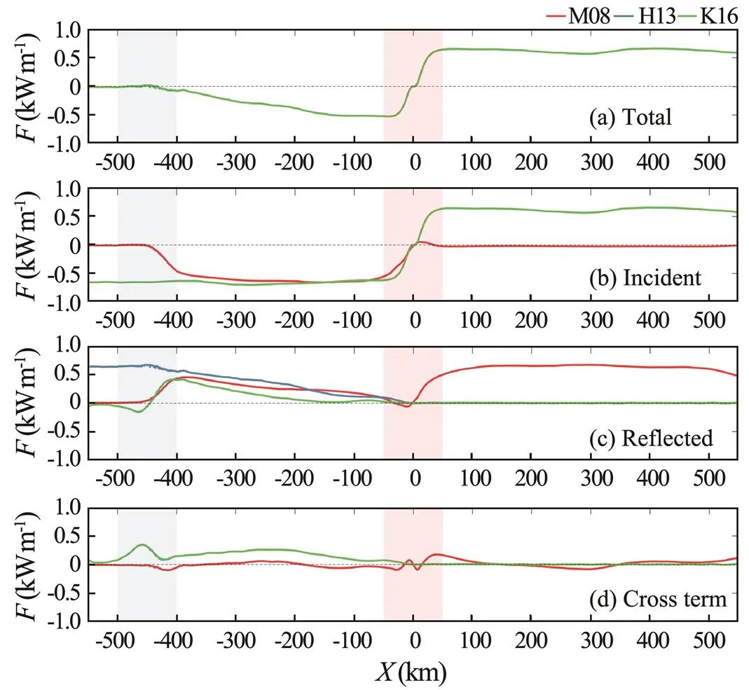
Fig.3 (a) Total, (b) incident, (c) reflected, and (d) cross term of the energy fluxes in case 2. Red, blue, and green curves denote results obtained by using the M08, H13, and K16 methods, respectively. The total energy fluxes shown in (a) are identical for the three methods, and the incident energy fluxes shown in (b) are identical for the H13 and K16 methods. In addition, no cross term of the energy flux exists in the H13 method. The blue shadings indicate the location of the slope, and the red shadings indicate the location of the Gaussian ridge.

3.3 Comparison Between the CELT Output and Extracted Results Using the M08 Method

In this section, the CELT is employed to solve case 2. The simulated results between the CELT and MITgcm have some differences. Since our aim is to validate the M08 method using the CELT calculation rather than comparing the CELT and MITgcm, such difference is beyond the scope of this study. Because the CELT directly outputs the total fields as well as eastward- and westward-propagating components of the simulated baro-clinic current and pressure perturbation (Kelly, 2013a), the data of this model can be used to assess the M08 method. To be specific, we use the M08 method to extract the incident (westward) and reflected (eastward) signals from the total fields of baroclinic current and pressure perturbation simulated by the CELT; the accuracy of the M08 method can then be validated by comparing the extracted signals with those outputted directly from the CELT.

Fig.4 shows the instantaneous baroclinic currents and pressure perturbations as well as the period-averaged energy fluxes calculated by using the M08 method and outputted directly from the CELT. No visual differences are observed between the eastward-propagating components of baroclinic current and pressure perturbation extracted by the M08 method and those outputted directly from the CELT. Thus, the incident (westward) and reflected (eastward) energy fluxes calculated by the M08 method and outputted directly from the CELT are identical, except in some small regions near the slope and Gaussian ridge. The slight differences observed could be attributed to the use of filtering in the M08 method, as explained above. Whereas, application of the H13 and K16 methods produces large biases in the results (Fig.5). The reflected energy fluxes are obviously underestimated by both methods. Between the two methods, the lower reflected energy flux is derived from the K16 method. Therefore, the M08 method is a feasible and accurate approach to separate the internal waves propagating in different directions. We note, however, that the signals extracted by this method may show slight bias in small regions near topographic features.

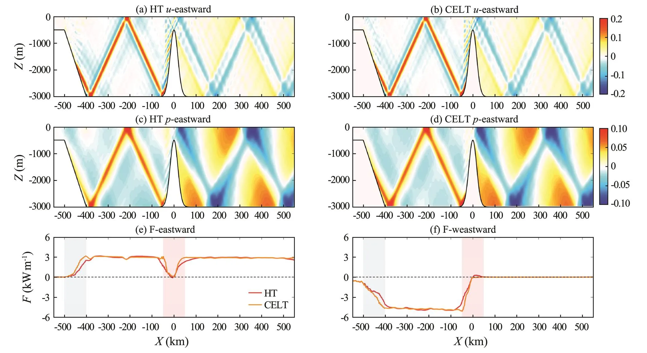
Fig.4 Eastward-propagating components of (a, b) the baroclinic current (unit: ms−1) and (c, d) pressure perturbation (unit: Pa) (a, c) extracted by the M08 method and (b and d) outputted directly from the CELT. (e) Eastward and (f) westward energy fluxes calculated by using the M08 method (red) and CELT output (yellow). The blue and red shadings indicate the locations of the slope and Gaussian ridge, respectively.

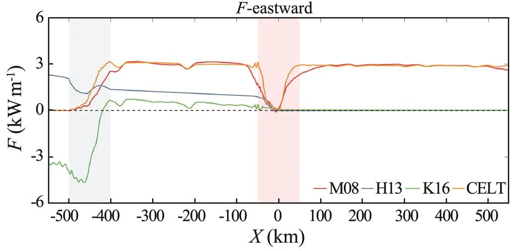
Fig.5 Eastward (reflected) K1 energy fluxes calculated by using the different methods (red, blue, and green lines) and the CELT output (yellow line). The blue and red shadings indicate the locations of the slope and Gaussian ridge, respectively.

3.4 Explanation for the Different Results of the Three Methods in Case 2

As the effectiveness and accuracy of the M08 method have been verified by comparison with the CELT calculations, the different results produced by the other methods in case 2 (Fig.3) should be interpreted. The first difference is that the incident energy fluxes extracted by the H13 and K16 methods are slightly larger than that extracted by the M08 method. The reason may be that in the H13 and K16 methods, the incident internal tides generated from the Gaussian ridge in the control run are inconsistent with those in case 2. In case 2, the incident internal tides generated from the Gaussian ridge are affected by internal tides generated upon the slope, whereas this effect is absent in the control run. Previous studies have shown that remotely generated internal tides can influence locally generated internal tides due to the phase difference between the current and pressure perturbation (Kelly and Nash, 2010; Kerry, 2013). Moreover, the interference of internal tides radiated from the two topographic features also affects the energy conversion, energy flux divergence, and dissipation of internal tides upon them (Buijsman, 2012, 2014). Fig.6 shows the K1energy fluxes in case 2 and the corresponding control run. As a comparison, the K1energy flux in the run where only the slope exists is also shown in Fig.6. The K1energy flux between the slope and Gaussian ridge (−400<<50km) in case 2 is much smaller than that in the control run, although the K1energy flux generated from the slope is very small. Following Buijsman(2012, 2014), the amplificationof the energy flux divergence at=±500km is calculated as

whererepresents the energy flux divergence at=±500km and subscripts ‘ridge+slope’, ‘ridge’ and ‘slope’ represent the case 2, the control run and the run considering the existence of the slope only. According to the energy flux divergence in the three runs (Fig.6),is approximately −0.5, suggesting a destructive interference (Buijs- man, 2012, 2014). In other words, the existence of the slope inhibits the generation of internal tides upon the Gaussian ridge.

The second difference is that the cross term of the energy flux calculated by using the K16 method is positive between the slope and the Gaussian ridge (−400<<50km) but nearly zero for the M08 method. This may be attributed to the inaccurate estimation of incident internal tides using the K16 method. It is reasonable that the cross term of energy flux along the gradient direction of the slope vanishes, which is consistent with the results of case 1, because the incident and reflected signals are out of phase due to their opposite propagating directions in the two-dimensional (-) situation. However, because the K16 method inaccurately estimates the incident signals (and), the calculatedandare also inaccurate and contain part of the incident signals. In other words, the incident and reflected signals are not out of phase. Therefore, the cross term of the energy flux estimated by the K16 method is not zero between the slope and Gaussian ridge in this case. Because the total energy fluxes are the same for the three methods, differences in the incident and cross term of the energy flux finally cause differences in the reflected energy fluxes.

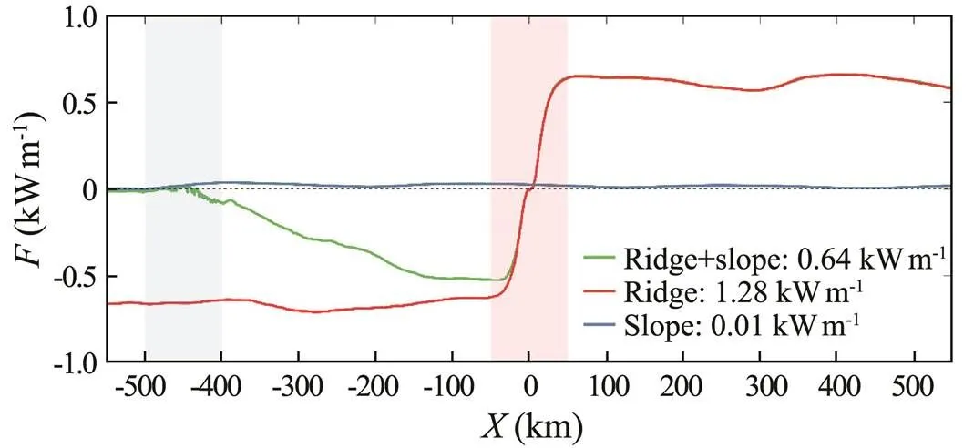
Fig.6 K1 energy fluxes in case 2 (green), the corresponding control run (red), and the run considering the existence of the slope only (blue). The green and red lines are overlap at the eastern portion of the Gaussian ridge (x>0km). The energy flux divergences at x=±500km are listed at the bottom right corner of the figure.

4 Summary

Reflection of internal tides on continental slopes is a common phenomenon in oceans, and it is crucial to the development of internal tide-driven turbulent mixing para- meterization on the slopes (MacKinnon, 2017) as the incident signals drive local turbulence (K16). In this work, the performances of three different methods (, M08, H13, and K16) in separating the reflected signals of internal tides from those of incident ones are determined, and the reflection of internal tides on slopes is investigated. The M08 method directly separates incident and reflected components from the total fields of baroclinic current and pressure perturbation based on the Hilbert transform, filtering, Fourier transform, and its inverse transform. By contrast, the H13 and K16 methods require a control run to determine the incident internal tide signals, and their difference is mainly manifested in the calculation of reflected energy fluxes. In this study, the applicability and accuracy of these methods are examined by comparing two different cases based on the simulated results of MITgcm and CELT.

In case 1 where westward mode-1 internal tides impact the slope, the three methods show similar performances and well capture the dynamic processes of internal tide reflection on the slope. However, in case 2, where internal tides are radiated from a Gaussian ridge and impact the slope, the H13 and K16 methods inaccurately estimates of the reflected energy fluxes because the westward-propagating components of baroclinic current and pressure perturbation in the control run are inconsistent with those in case 2. In other words, the incident signals of internal tides estimated by the H13 and K16 methods are inaccurate. By contrast, the M08 method can accurately estimate for both incident and reflected internal tides. However, although the M08 method based on the Hilbert transform is more suitable than the two other methods for both cases considered in this study, it should be noted that this method can result in slight bias when separating incident and reflected signals near topographic features due to its use of filtering.

Acknowledgements

This study is supported by the National Key Research and Development Program (No. 2017YFA0604103), the National Program on Global Change and Air-Sea Interaction (No. GASI-IPOVAI-04), the National Natural ScienceFoundation of China (Nos. 41806012, 41876015, and 41576008), and the Fundamental Research Funds for the Central Universities. The authors would like to thank Dr. Samuel M. Kelly for sharing the code of the CELT. Insightful discussions with Dr. Qun Li are gratefully appreciated.

Alford, M. H., 2003. Redistribution of energy available for ocean mixing by long-range propagation of internal waves., 423 (6936): 159.

Baines, P. G., 1982. On internal tide generation models., 29 (3A): 307-338.

Bell, T. H. J., 1975. Topographically generated internal waves in the open ocean., 80 (3): 320-327.

Buijsman, M. C., Klymak, J. M., Legg, S., Alford, M. H., Farmer, D., Mackinnon, J. A., Nash, J. D., Park, J., Pickering, A., and Simmons, H., 2014. Three-dimensional double-ridge internal tide resonance in Luzon Strait., 44 (3): 850-869.

Buijsman, M. C., Legg, S., and Klymak, J., 2012. Double-ridge internal tide interference and its effect on dissipation in Luzon Strait., 42 (8): 1337-1356.

Carter, G. S., Fringer, O. B., and Zaron, E. D., 2012. Regional models of internal tides., 25 (2): 56-65.

Chen, Z., Xie, J., Xu, J., He, Y., and Cai, S., 2017. Selection of internal wave beam directions by a geometric constraint provided by topography., 29 (6): 066602.

Dauxois, T., Didier, A., and Falcon, E., 2004. Observation of near-critical reflection of internal waves in a stably stratified fluid., 16 (6): 1936.

Garrett, C., 2003a. Oceanography: Mixing with latitude., 422 (6931): 477-478.

Garrett, C., 2003b. Internal tides and ocean mixing., 301 (5641): 1858-1859.

Ghaemsaidi, S. J., Joubaud, S., Dauxois, T., Odier, P., and Peacock, T., 2016. Nonlinear internal wave penetrationparametric subharmonic instability., 28 (1): 011703.

Hall, R. A., Huthnance, J. M., and Williams, R. G., 2013. Internal wave reflection on shelf slopes with depth-varying stratification., 43 (2): 248-258.

Kelly, S. M., and Nash, J. D., 2010. Internal-tide generation and destruction by shoaling internal tides., 37 (23): 817-824.

Kelly, S. M., Jones, N. L., and Nash, J. D., 2013a. A coupled model for Laplace’s tidal equations in a fluid with one horizontal dimension and variable depth., 43 (8): 1780-1797.

Kelly, S. M., Jones, N. L., Nash, J. D., and Waterhouse, A. F., 2013b. The geography of semidiurnal mode-1 internal-tide energy loss., 40 (17): 4689-4693.

Kerry, C. G., Powell, B. S., and Carter, G. S., 2013. Effects of remote generation sites on model estimates of M2internal tides in the Philippine Sea., 43 (1): 187-204.

Klymak, J. M., Alford, M. H., Pinkel, R., Lien, R. C., Yang, Y. J., and Tang, T. Y., 2011. The breaking and scattering of the internal tide on a continental slope., 41 (5): 926-945.

Klymak, J. M., Simmons, H. L., Braznikov, D., Kelly, S., Mac- kinnon, J. A., Alford, M. H., Pinkel, R., and Nash, J. D., 2016. Reflection of linear internal tides from realistic topography: The Tasman continental slope., 46 (11): 3321-3337.

Kunze, E., Rosenfeld, L. K., Carter, G. S., and Gregg, M. C., 2002. Internal waves in Monterey submarine canyon., 32 (6): 1890-1913.

Legg, S., 2014. Scattering of low-mode internal waves at finite isolated topography., 44: 359-383.

Legg, S., and Adcroft, A., 2003. Internal wave breaking at concaveandconvexcontinentalslopes., 33 (11): 2224-2246.

MacKinnon, J. A., Zhao, Z., Whalen, C. B., Waterhouse, A. F., Trossman, D. S., Sun, O. M., St. Laurent, L. C., Simmons, H. L., Polzin, K., Pinkel, R., Pickering, A., Norton, N. J., Nash, J. D., Musgrave, R., Merchant, L. M., Melet, A. V., Mater, B., Legg, S., Large, W. G., Kunze, E., Klymak, J. M., Jochum, M., Jayne, S. R., Hallberg, R. W., Griffies, S. M., Diggs, S., Danabasoglu, G., Chassignet, E. P., Buijsman, M. C., Bryan, F. O., Briegleb, B. P., Barna, A., Arbic, B. K., Ansong, J. K., and Alford, M. H., 2017. Climate process team on internal wave-driven ocean mixing., 98 (11): 2429-2454.

Marshall, J., Adcroft, A., Hill, C., Perelman, L., and Heisey, C., 1997. A finite-volume, incompressible Navier-Stokes model for studies of the ocean on parallel computers., 102 (C3): 5753-5766.

Martini, K. I., Alford, M. H., Kunze, E., Kelly, S. M., and Nash, J. D., 2011. Observations of internal tides on the Oregon continental slope., 41 (9): 1772-1794.

Martini, K. I., Alford, M. H., Kunze, E., Kelly, S. M., and Nash, J. D., 2013. Internal bores and breaking internal tides on the Oregon continental slope., 43 (1): 120-139.

Mathur, M., Carter, G. S., and Peacock, T., 2014, Topographic scattering of the low-mode internal tide in the deep ocean., 119: 2165-2182.

Mercier, M. J., Garnier, N. B., and Dauxois, T., 2008. Reflection and diffraction of internal waves analyzed with the Hilbert transform., 20 (8): 322-636.

Mercier, M. J., Gostiaux, L., Helfrich, K., Sommeria, J., Viboud, S., Didelle, H., Ghaemsaidi, S. J., Dauxois, T., and Peacock, T., 2013. Large-scale, realistic laboratory modeling of M2internal tide generation at the Luzon Strait., 40 (21): 5704-5709.

Muller, P., and Liu, X. B., 2000. Scattering of internal waves at finite topography in two dimensions. Part I: Theory and case studies., 30 (3): 532-549.

Munk, W., and Wunsch, C., 1998. Abyssal recipes II: Energetics of tidal and wind mixing., 45 (12): 1977-2010.

Nash, J. D., Alford, M. H., and Kunze, E., 2005. Estimating internal wave energy fluxes in the ocean., 22 (10): 1551-1570.

Nash, J. D., Kunze, E., Toole, J. M., and Schmitt, R. W., 2004. Internal tide reflection and turbulent mixing on the continental slope., 34 (5): 1117-1134.

Nie, Y., Chen, Z., Xie, J., Xu, J., He, Y., and Cai, S., 2019. Internal waves generated by tidal flows over a triangular ridge with critical slopes., 18: 1005-1012.

Peacock, T., Mercier, M. J., Didelle, H., Viboud, S., and Dauxois, T., 2009. A laboratory study of low-mode internal tide scattering by finite-amplitude topography., 21 (12): 121702.

Rainville, L., and Pinkel, R., 2006. Propagation of low-mode internal waves through the ocean., 36 (6): 1220-1236.

Ray, R. D., and Mitchum, G. T., 1996. Surface manifestation of internal tides generated near Hawaii., 23: 2101-2104.

Rudnick, D. L., Boyd, T. J., Brainard, R. E., Carter, G. S., Egbert, G. D., Gregg, M. C., Holloway, P. E., Klymak, J. M., Kunze, E., Lee, C. M., Levine, M. D., Luther, D. S., Martin, J. P., Merrifield, M. A., Moum, J. N., Nash, J. D., Pinkel, R., Rainville, L., and Sanford, T. B., 2003. From tides to mixing along the Hawaiian ridge., 301 (5631): 355-357.

Sutherland, B. R., Keating, S., and Shrivastava, I., 2015. Transmission and reflection of internal solitary waves incident upon a triangular barrier., 775: 304-327.

Wang, S., Chen, X., Li, Q., Wang, J., Meng, J., and Zhao, M., 2018a. Scattering of low-mode internal tides at different shaped continental shelves., 169: 17-24.

Wang, S., Chen, X., Wang, J., and Meng, J., 2018b. Experimental investigation of internal tides generated by finite-height topography., 68: 957-965.

Wang, S., Chen, X., Wang, J., Li, Q., Meng, J., and Xu, Y., 2019. Scattering of low-mode internal tides at a continental shelf., 49 (2): 453-468.

Wang, Y., Xu, Z., Yin, B., Hou, Y., and Chang, H., 2018c. Long-range radiation and interference pattern of multi-source M2internal tides in the Philippine Sea., 123: 5091-5112.

Wu, L., Miao, C., and Zhao, W., 2013. Patterns of K1and M2internal tides and their seasonal variations in the northern South China Sea., 69 (4): 481-494.

Xu, Z., Liu, K., Yin, B., Zhao, Z., Wang, Y., and Li, Q., 2016. Long-range propagation and associated variability of internal tides in the South China Sea., 121 (11): 8268-8286.

Zhao, Z., 2017. The global mode-1 S2internal tide., 122 (11): 8794-8812.

Zhao, Z., Alford, M. H., Girton, J. B., Rainville, L., and Simmons, H. L., 2016. Global observations of open-ocean mode-1 M2internal tides., 46 (6): 1657-1684.

Zhao, Z., Alford, M. H., Mackinnon, J. A., and Pinkel, R., 2010. Long-range propagation of the semidiurnal internal tide from the Hawaiian ridge., 40 (4): 713-736.

. E-mail: caoanzhou@zju.edu.cn

July 23, 2019;

December 4, 2019;

December 16, 2019

(Edited by Xie Jun)