Performances of Clustering Methods Considering Data Transformation and Sample Size: An Evaluation with Fisheries Survey Data

WO Jia, ZHANG Chongliang, XU Binduo, XUE Ying, and REN Yiping, 2), *

Performances of Clustering Methods Considering Data Transformation and Sample Size: An Evaluation with Fisheries Survey Data

WO Jia1), ZHANG Chongliang1), XU Binduo1), XUE Ying1), and REN Yiping1), 2), *

1),,266003,2),,266237,

Clustering is a group of unsupervised statistical techniques commonly used in many disciplines. Considering their applications to fish abundance data, many technical details need to be considered to ensure reasonable interpretation. However, the reliability and stability of the clustering methods have rarely been studied in the contexts of fisheries. This study presents an intensive evaluation of three common clustering methods, including hierarchical clustering (HC), K-means (KM), and expectation-maximization (EM) methods, based on fish community surveys in the coastal waters of Shandong, China. We evaluated the performances of these three methods considering different numbers of clusters, data size, and data transformation approaches, focusing on the consistency validation using the index of average proportion of non-overlap (APN). The results indicate that the three methods tend to be inconsistent in the optimal number of clusters. EM showed relatively better performances to avoid unbalanced classification, whereas HC and KM provided more stable clustering results. Data transformation including scaling, square-root, and log-transformation had substantial influences on the clustering results, especially for KM. Moreover, transformation also influenced clustering stability, wherein scaling tended to provide a stable solution at the same number of clusters. The APN values indicated improved stability with increasing data size, and the effect leveled off over 70 samples in general and most quickly in EM. We conclude that the best clustering method can be chosen depending on the aim of the study and the number of clusters. In general, KM is relatively robust in our tests. We also provide recommendations for future application of clustering analyses. This study is helpful to ensure the credibility of the application and interpretation of clustering methods.

hierarchical cluster; K-means cluster; expectation-maximization cluster; optimal number of clusters; stability; data trans- formation

1 Introduction

With the increasing impacts of climate changes, over- fishing, and other human activities, worldwide marine eco- systems have been facing with substantial habitat fragmen- tation and the formation of patches of communities (Jack- son, 2001). Such fragmentation of ecosystems has a critical impact on marine conservation and management, as the patches or ecoregions are often characterized by different biotic communities and need to be studied ex- tensively (Okubo, 2006; Valentine-Rose, 2007; Pais, 2013). As a matter of practicality, there is a growing demand for statistical methods to identify biotic communities and ecoregions for the successful imple- mentation of conservation plans (Wikramanayake, 2002; Ricketts and Imhoff, 2003; Giakoumi, 2013).

Analyses of biotic community data usually depend on multivariate statistics, which are now widely accepted by ecologists to detect and describe different patterns ac- cording to many variables (Tabachnick, 2007). The most common multivariate problem in marine ecology is to develop the methods of classification according to com- munity structure, climate variation, and spatial distribution. As a typical and popular classification method, clustering analysis is most widely applied in ecology, particularly in benthic and plankton communities (Cao, 1997; Xi, 1997; Ysebaert, 2003; Doherty, 2010; Ri- chter, 2015; Wang, 2018). It is mainly used to define homogeneous regions with ecological or manage- ment objectives (Green, 1980). Technically, cluster analy- sis is one type of unsupervised learning method that does not tag objects with prior identifiers, as opposed to some classification, discriminant analysis, and supervised learn- ing methods. It can help identify underlying structures in data and help understand how survey locations differ in terms of species composition without explicit reference to explanatory variables (Ysebaert, 2003). Therefore, as an exploratory tool, clustering methods could guide in identifying ecoregions. Nevertheless, although clustering often yields simple and interpretable results, the adequacy of the solutions is rarely evaluated in practice (Clarke, 2016).

There are diverse clustering methods, which differ in theories and math methods. Most of them are algebra-based and involve applying a series of algebraic operations to a matrix of pairwise dissimilarities. The algebra-based clustering algorithms can be broadly divided into two groups: hierarchical and partitional approaches, which in- clude hierarchical clustering (HC) and K-means (KM) clus- tering, respectively, while the development of new tech- niques is still an ongoing research area (Li, 2008; Sutherland, 2012; Wang, 2012). Meanwhile, a different clustering approach, namely model-based clus- tering, adopts the density function in the form of prob- abilistic mixture models. This approach assumes that data are generated from a mixture distribution, and each cluster is described by one or more mixture components (Lindsay, 1989). Differing from the algebra-based methods, model-based methods may be useful to tackle irregular data and incorporate diverse distributional patterns, such as gamma, negative binomial, and Tweedie distributions. By far, model-based clustering methods have received less attention in ecology, and only in recent years has there been progress from methodology to application (Dunstan and Bushby, 2013; Hui, 2017).

The availability of many clustering methods makes it necessary to evaluate and compare them for practical pur- poses (Pais, 2013; Hui, 2017). Moreover, the grow- ing diverse types of datasets also contribute to the wide use of clustering algorithms, while the guidelines for their app- lications are important. Preliminarily, a tactical problem of clustering is determining the suitable methods, as different algorithms often result in entirely different partitions on the same data. In addition, the uses of clustering have com- monly involved a certain level of arbitrariness (Clarke, 2016), which imposes considerable issues in the different partitions interpretation; for example, the number of mean- ingful clusters (referred to as K) is often subjective in the view of stockholders, and this substantially undermines the confidence in clustering methods and hampers their application in management decision. These issues have re- sulted in publications focusing on comparative studies in the recent bioinformatics and computational biology lit- erature (Khondoker, 2016). Although clustering ana- lysis is widely applied in ecology, especially fisheries (Xi, 1997), the relationship between the analysis me- thods and the characteristics of data has been rarely tested and is not well understood. Furthermore, transforming the original data is a common practice, for instance, trans- forming abundance/biomass to a log- or square-rooted scale in order to adjust the skewed distribution and satisfy the assumption of inferential statistics (Templ., 2008); however, the pre-treatment process may lead to informa- tion loss and changes in data structure. Another issue of clustering is its robustness to the stochasticity of survey data (Datta and Datta, 2003; Clarke, 2016), as sample size may influence the clustering performance (Markovic, 2013). Therefore, when choosing clustering methods for practical use, data transformation types and the size of survey data should be among the primary considerations.

In this study, three clustering methods are selected re- garding their convenient usages and wide applications in fisheries studies, and their performances in identifying community structures based on the fisheries survey data in the Yellow Sea, China, are evaluated. As fish abundance data are usually right-skewed (Vaudor, 2011), data transformation was conducted before clustering analyses. We evaluated three common clustering technologies: hi- erarchical clustering (HC), K-means (KM) clustering, and expectation-maximization (EM) clustering (Lloyd, 1982; Li and Xu, 2007; Jin and Han, 2016), considering different data transformation methods and data sizes. Diverse cri- teria are used to determine the optimal number of clusters, and a stability index is used to measure the robustness of the clustering methods to the stochasticity in survey data. This study aims to contribute to the further clarification and credible applications of clustering methods in reveal- ing ecoregions, and support adaptive strategies of fisheries management in patched marine ecosystems.

2 Materials and Methods

2.1 Survey Data

The studied area is located in the coastal waters of the North Yellow Sea (NYS), off Shandong Province (35.00˚– 39.00˚N, 119.40˚–124.00˚E). The position is shown in Fig.1. A bottom trawl survey was conducted in the fall of 2016 to collect data on species composition and fish distribu- tions. A total of 118 sites were investigated, using otter trawl vessels of 161.8kW and a trawl net with a width of 25m and mesh size of 17mm (Fig.1). The relative abundance of fish by species was calculated as the catch in weight di- vided by fishing efforts, 2knot×hour (trawling speed×time), and with the unit of ‘g(nautical mile)−1’. As fisheries data often include very large observations, which might large- ly impact the clustering results, three data transformation methods, scaling/standardization (scale), square-root (sqrt), and log-transformation (log), were applied before cluster- ing analyses to adjust the skewed distribution in fishery (Templ, 2008). Fishes were identified, counted, and measured, and only species with over five individuals were selected for analyses. Fish abundance in the NYS survey was referred to as the ‘survey data’ in the clustering ana- lyses.

Fig.1 Study area and sampling sites in the coastal waters of the North Yellow Sea.

2.2 Clustering Methods

Clustering techniques are aimed to group the survey sites into clusters that are both well separated and homogeneous as much as possible considering the observation abun- dance. The characteristics of survey data used in this study were fish community composition, that is, the relative abun- dance (catch per unit effort) of each species. We used three types of clustering methods to analyze the survey data of fish community: two algebra-based methods and one mo- del-based method. The three clustering methods were im- plemented on the community abundance from fisheries sur- veys, with species abundance as targeted variables and sam- pling sites as samples or observations (Fig.1). The threeclustering methods are briefly introduced below.

1) Hierarchical clustering (HC)

Hierarchical clustering (HC) is the most well-known and frequently used clustering algorithm (Kaufman and Rous- seeuw, 1990). This method generates a partition tree or a dendrogram that shows a clear-cut cluster in a two-dimen- sional plot. Technically, samples start in a separate cluster and successively join together in terms of the closeness of distance, determined by a dissimilarity measurement. Based on the similarity matrix, a clustering linkage method is used to obtain a taxonomic hierarchy in the form of a den-drogram (McCabe, 1975). We used a common lin- kage option known as the unweighted pair group method with arithmetic mean (UPGMA) combined with Euclidean distance (and many other distances available) to determine the closeness between clusters. The UPGMA derives an equivalence matrix from the given similarity matrix (Daw- yndt, 2006). We applied HC with the base R function ‘hclust’.

2) K-means (KM) clustering

The KM algorithm is also one of the most popular clustering algorithms (Lloyd, 1982). As a center-based tech-nique, the KM, which is only appropriate for Euclidean distance matrices, aims to find partitions such that the residual squared error within the points of a cluster is mi- nimized. The KM is defined so that the minimum residual values are considered indicative of a desirable set of clusters. It differs from HC in that the solution does not portray a hierarchical structure and the number of clusters () must be specified in advance (Everitt, 1980). The main steps of the KM algorithm are as follows: i) select an initial parti- tion withclusters; ii) generate a new partition by as- signing each point to its closest cluster center; and iii) re- peat to generate new clusters until cluster membership sta- bilizes. The mean value of the data points of are calculated using the same ‘average distance’ as in HC and implement-ed with the R function ‘K-means’.

3) Expectation-maximization (EM) clustering

The EM clustering is a model-based clustering method (Kushary, 2012) in which clusters are defined based on how likely the objects belong to the same distribution. Model-based clustering is computationally expensive for high-dimensional data (James and Sugar, 2003). Compared with KM, which assumes all clusters are spherical (equal variance-covariance), EM allows clusters to have different variances, densities, and sizes (Peña, 2018). The algorithm includes two steps: expectation and maximization. The ex- pectation step requires the computation of the predicted values of an unobserved latent variable, while in the ma- ximization step, the objective function, given by the like- lihood of underlying latent processes, is maximized over the admissible parameter space (Valter and Marcello, 2008). Moreover, the algorithm is constrained with a specific num- ber of Gaussian distributions to overcome overfitting (Gau- ssian mixture models). The EM is implemented in the ‘model-based clustering’ function in the R package ‘mclust’.

A variety of metrics can be used to calculate the distance between observations for the HC and EM clusters, whereas only Euclidean distance is applicable for KM (Jain, 2004). To make the methods comparable, Euclidean dis- tance is adopted for all methods in this study (Clarke, 2016). The relative abundance of all species was used to calculate the Euclidean distance among sampling sites (observation). This pairwise Euclidean distances between sampling sites were used as similarity indices to conduct cluster analyses. The original data matrix of abundance is arranged with species in columns and stations in rows. Meanwhile, it should be noted that different distance me- thods may result in distinct results in different sample sizes and transformations.

2.3 Determine the Number of Clusters

Choosing the proper number of clusters () is critical for the interpretation of clustering methods, especially for KM. Taking the survey area of this study for example, the fish community is located in both coastal and offshore waters of north and south regions (Fig.1); therefore, a clus- ter number of two to four should be reasonable according to the geographic layout. This study used the measures of connectedness and separation in cluster partitions, includ- ing ‘elbow’, ‘silhouette’, and Bayesian information criterion (BIC), among many cluster validity indices (CVIs) (Mil- ligan and Cooper, 1985).

1) Within-cluster sums of squares: The total within-cluster sum of squares (WSS), also referred to as ‘elbow’, features one of the most common CVI variance curves. The WSS measures the compactness of clustering, and a small value indicates high compactness and satisfactory clustering results. We display the curve showing the changes of WSS with differents, in which the location of a bend (knee) is generally considered as an indicator of the ap- propriate number of clusters (Thorndike, 1953).

2) Average silhouette: Silhouette is a measure of the closeness of data within a cluster and the looseness of data among neighboring clusters (Rousseeuw, 1987). Therefore, the average silhouette method measures the quality of clus- tering by determining how well each object lies within its cluster,

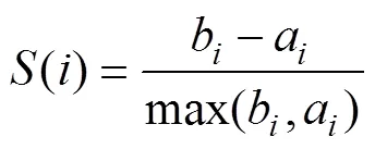
where() is the silhouette of data sample/observation;ais the average distance betweenand all other observations in the same cluster; andbis the average distance betweenand the observations in the ‘nearest neighboring cluster’. Additionally,() is the cluster containing observation;() is the cardinality of cluster;Cis the ‘nearest neigh- boring cluster’ of(); dist(,) is the distance between ob- servationsand, measured by the Euclidean distance. The optimal number of clusters () is the one that maximizes the average silhouette over a range of possible values (Kau-fman and Rousseeuw, 1990).

3) Bayesian information criterion (BIC): Theis an approximation to the Bayes factor (Schwarz, 1978), which adds a penalty to the log-likelihood based on the number of parameters.

We used the elbow and silhouette indices to decide the optimalfor HC and KM, and usedfor EM. For all cases, we evaluated the three CVIs with candidate clustersranging from 2 to 10. The BIC is calculated in the ‘Mclust()’function in the mclust package. The ‘fviz_nbclust()’ func- tion statement in the R package ‘factoextra’ was used to cal-culate the elbow and silhouette indices (Kassambara and Mundt, 2016).

2.4 Performance Evaluation

1) The average proportion of non-overlap: The robust- ness of clustering methods should be considered as a matter of practicability since survey data are vulnerable to errors and stochastic processes in observation. To simulate these scenarios and evaluate the stability of the clustering methods, herein, we implemented a delete-one jackknife approach to calculate the index of average proportion of non-overlap (APN) (Pearson, 2010; Brock, 2011). The approach involves measuring the average proportion of observations not placed in the same cluster after eli- minating one observation. It allows labels changing in the outcome, whereas thedoes not change. That is, we repeated clustering algorithms for the dataset by deleting the observation at site=1, 2, 3, …,each time.

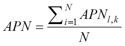
2) Pielou’s evenness index (J): Sometimes clustering results may be severely asymmetrical; that is, some parti- tions may contain a few observations and others may con- tain more, which, however, tend to be meaningless and should be avoided for ecoregions identification. The Pielou’s evenness index was generalized to quantify evenness and calculated by the following equation (Pielou, 1966):

whereis the total number of clusters,Pis the proportion of the number of sites in clusterto the total number of sites, and′ is the Shannon-Wiener diversity index.

The stability and evenness were evaluated for the three clustering methods. Additionally, we considered the influ- ences of data transformation on cluster results for cluster numbers ranging from 2 to 10. Three commonly used ap- proaches of data transformation–scaling, log, and square-rooted transformations–were adopted before clustering analyses. Moreover, considering the important role of the sample size in clustering methods, for the three clustering methods, we used the bootstrap approach to test the ro- bustness (APN) to sample size. That is, we simulated a new dataset with the same number of species but varying sample sizes, from 50 to 100 survey stations, randomly drawn from the original dataset. The processes were re- peated 1000 times for each clustering method and sample size.

3 Results

3.1 Optimal Number of Clusters

Different clustering methods and discriminant criteria led to a varying number of clusters. According to the elbow and silhouette criteria,=2 was the suitable num- ber for log-transformation data in HC and KM clustering. According to thetrends,=6 was the appropriate number in EM (Fig.2), and three optimal cluster results (HC, KM, and EM) are shown in Fig.3. In addition, data transformations led to a substantial difference in the se- lection offor HC, KM and EM clustering (Table 2). For HC and KM, the resultantwas stable, ranging from 2 to 3, whereas for EM clustering, the estimatedwas 3, 6, and 2 in the scale-, log- and sqrt-transformations, respecttive- ly. The number of sampling sites tended to be asymme- trical in HC and KM; for example, scaled data led to two clusters, including 1 and 117 sites, log-data led to 35 and 83 sites, and sqrt data led to 5 and 113 sites in KM clustering.

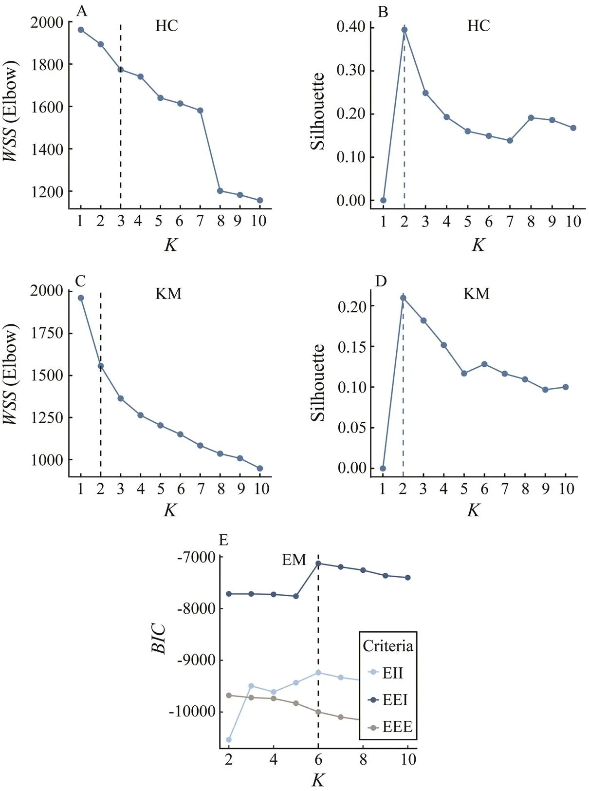
Fig.2 The optimal number of clusters in HC, KM and EM clustering based on the same data. Elbow and silhouette criteria were used for HC and KM, and BIC was used for EM.

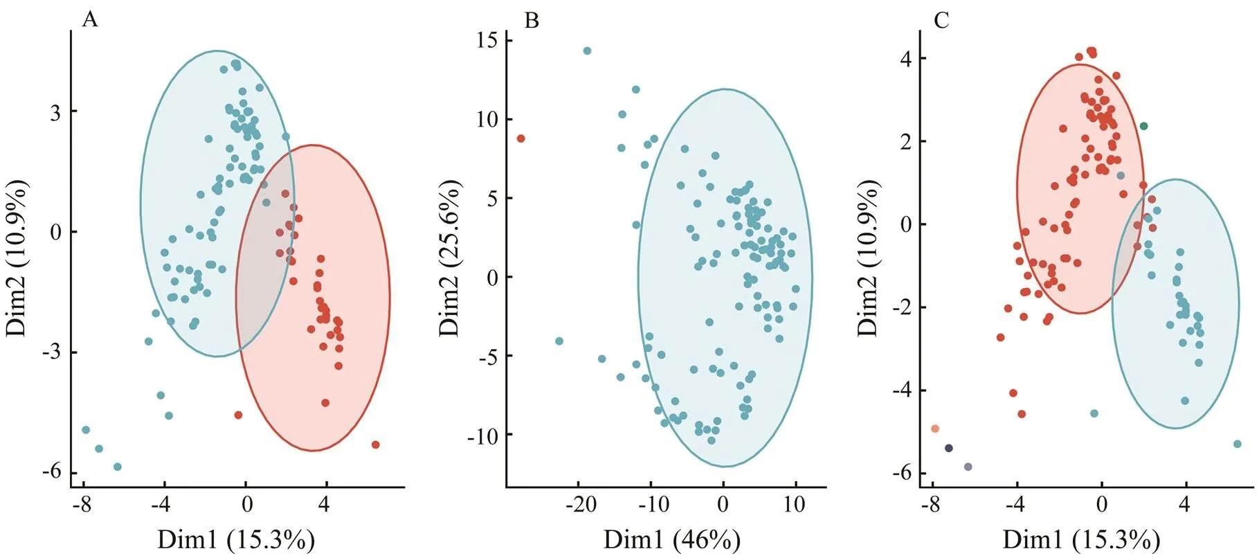
Fig.3 The optimal clustering results after log-transformation: (A) HC, (B) KM clustering, and (C) EM clustering. Different clusters are distinguished by the colors of points. The axis was derived from principal component analysis, where the x-axis represents PC1, and the y-axis represents PC2, and the values denote the score of the principal components.

Table 1 The details of clustering parameterization to evaluate the impacts of different combinations

Table 2 The optimal number of clusters considering different ways of data transformation

3.2 Evenness and Stability of Clustering

Pielou’s index was used to evaluate the evenness and avoid the asymmetry of the clustering results. In general, the three clustering methods showed varying levels of even- ness in their results, depending on the number of clusters and types of data transformation. Among them, KM show- ed the best evenness with log-transformation, and EM had fair performances of evenness with the other types of trans-formation, especially for smalls (Fig.4). HC showed the least performance on evenness among the three clustering methods.

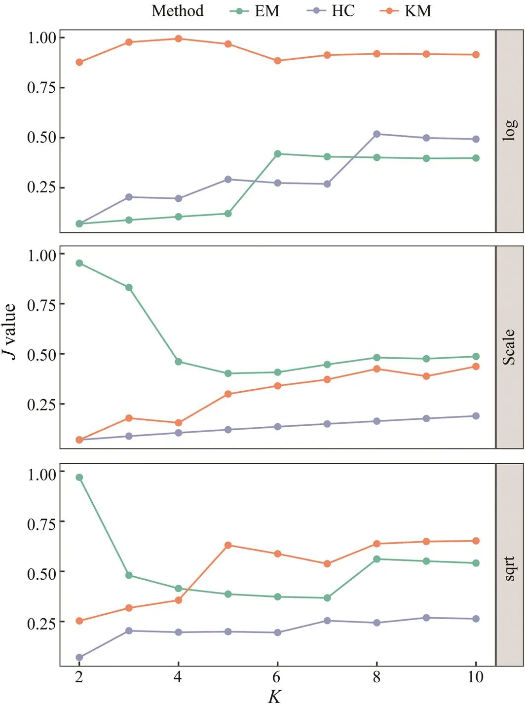
Fig.4 Performance of the evenness (J) of clustering results as the K value is increased. The three plots correspond to three data pre-treatment approaches, and the colored lines indicate three cluster algorithms.

We further evaluated the stability of clustering with re- spect to different data transformation approaches and cluster numbers. The clustering methods showed a different res- ponse to data transformation: HC had a low level of APN in all three transformations; KM was more stable with scaling; and EM showed better performance with log-trans-formation. In general, scaled data tended to provide a more stable solution at the same cluster number. Additionally, KM tended to decrease in stability with increasing, EM showed the opposite trend, and HC was barely influenced by the choice of. According to the selection criteria in 3.1, we compared the stability of each combination with respect to the optimalvalue (HC=3,KM=2,EM=6) (Fig.5) after applying log-transformation. In this case, HC and KM provided stable results with a low APN; in par- ticular, KM with two clusters provided a very small value. The stability of EM clustering was much less than those of the other two.

Fig.5 Performance of average proportion of non-overlap (APN) of clustering results with increase in K value. The three plots correspond to three data pre-treatment ap- proaches, and the colored lines indicate three cluster algo- rithms.

The two performance indices, Pielou’s evenness () and stability index, showed a certain level of correlation in our evaluation (Fig.6). In general, the correlation was positive with a correlation coefficient=0.47 over the three clustering methods (<0.01), indicating the tradeoff between the stability and evenness of clustering results. However, the correlations also varied among clustering methods; that is, KM showed a strong correlation (=0.48,<0.05) and EM showed insignificant results (=−0.14,>0.1).

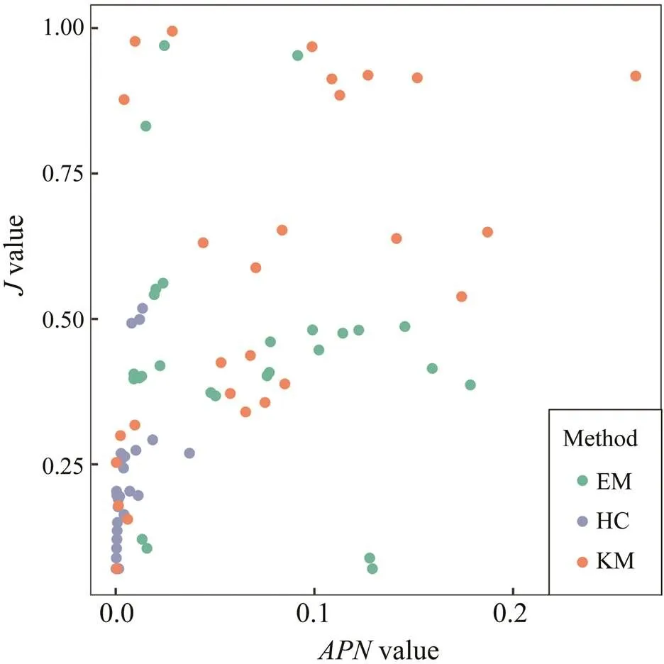
Fig.6 The correlation between APN and Pielou’s evenness index (J) in cluster analyses. Each point in the figure cor- responds to the results derived from Fig.4 (same as Fig.5).

3.3 The Effect of Sample Size

To evaluate the effects of sample size, we compared the clustering stability of resampled data with different sample sizes ranging from 50 to 100. Clustering with log-transfor- mation was performed using the optimalvalue (HC=3,KM=2,EM=6) (Fig.3). For all cluster methods,va- lues decreased with increasing sample sizes, indicating improved stability (Fig.7). However, the changing rates ofleveled off over 70 samples in general, depending on the clustering methods. The EM reached stable values at about 60 sites, while KM showed slight decreases be- tween 70 and 75 sites. HC clustering was relatively less res- ponsive to the increase of data sizes.

Fig.7 Performance of stability (APN) of clustering results with increase in data size. The three plots correspond to three cluster algorithms, and the colored shades indicate 95% confidence intervals.

4 Discussion

Validation is a vital issue to the success of clustering applications (Smith and Jain, 1988; Maulik and Bandyo- padhyay, 2002). To evaluate the credibility in their usage, the present study applies three common clustering meth- ods to the survey data of a fish community, and the eva- luations demonstrated that the performances of the clus- tering methods are substantially influenced by different factors, including the number of clusters, data transforma- tion, sample size, and algorithm selection. Given that clus- tering analysis has been a common practice in biotic com- munity research, such a pattern should be noted for future studies and practices. Therefore, we highlight that the in- terpretation of clustering methods requires domain know- ledge (Jain, 2008), and choosing proper methods and prior structure of the data and setups are the key to reasonable conclusions.

The stability of clustering methods is a major focus of this work. The topic has been covered in previous studies, in areas such as acoustic image clustering (Peña, 2018), image processing (Jain and Chen, 2004), computer science, and biological gene identification (Datta and Datta, 2003). As a recent example, Clarke(2016)showed that con- sistent grouping might result from three different cluster- ing methods in a zooplankton dataset, indicating the proper robustness of those methods. Another evaluation study with acoustic data has shown that EM clustering is a more ro- bust technique than KM in separating acoustic signatures and noise (Peña, 2018). However, these conclusions are different from ours. Our studies showed the substantial dif-ferences among clustering methods and a relatively low stability of EM. Such differences might be caused by the specific characteristics of different fisheries data. Due to the complex interactions between fish behaviors and fish- ing operation, fisheries surveys are usually affected by sub-stantially varying catchability (Arreguín-Sánchez, 1996), which is subjective to inevitable size selectivity and is less representative to population size. Therefore, it is common in fisheries that abundance data are highly skewed, as many of them are very small or zeros, and a few are extremely large, resulting in statistical problems in adopting many multivariate methods. Furthermore, as a soft-membership clustering technique, EM clustering may result in less stable solutions because it allows clusters to have different sizes and statistical distributions. Therefore, our study demon- strates that the results of clustering, especially EM, may be highly unstable with respect to the survey data of fish communities and that the influence of the irregularity of fishery data needs to be well understood in multivariate analyses procedure. As a fundamental issue to interpret cluster results, the stability or consistency of clustering pa- rameterization must be evaluated in advance.

Another concern in this study is the determination of the optimal number of clusters. Given that neither hierarchical nor partition methods directly address this issue (Fraley and Raftery, 1998), one advantage of EM clustering is that it selects not only the parameterization of the model but also the number of clusters simultaneously using appro- ximate Bayes factors. On the other hand, additional ana- lyses are needed to determine the number of clusters for HC and KM, which, however, may lead to inconsistent re- sults according to our evaluation. Nevertheless, similar research has rarely been conducted in fisheries studies. In such a case, experience and background knowledge are needed to find meaningful ecological partitions in spite of statistical techniques.

Regarding the common purpose of clustering analyses for indicating ecoregions in marine management, we sug- gest that the evenness of clustering results should be con- sidered in the selection and evaluation of algorithms in combination with the results stability (Altman and Krzy- winski, 2017). Although the cluster validity indices(CVIs) ‘elbow’ and ‘silhouette’ provided an approximate result, the two clustering groups in both HC and KM tended to be meaningless by dividing the survey areas into partitions of 1 and 117 sites. The group with only one survey site is com-monly treated as an outlier as a result of observation errors and is removed from the dataset for meaningful interpre- tation of community structure. However, the issue cannot easily be eliminated from our study, as removing the cur- rent ‘outlier’ tends to result in new ‘outliers’ and conse- quently a new asymmetric result with a cluster/group that contains only one site. The irregularity of the specific fish- eries data may contribute to the undesirable performances of clustering methods, which need to be accounted for with further improved clustering algorithms and distance mea- sures (Jain and Chen, 2004). Moreover, the different ob- jectives of studies can cause different results; for example, an asymmetric grouping with outliers might be meaningful for identifying dominant or rare species, but less mean- ingfulfor ecoregions identification.

The third concern in this study is that different pre-treatment procedures lead to different stabilities and in- terpretabilities of the clustering output. Specifically, traw- ling surveys usually lead to largely irregular distributions in fisheries data, such as inflated zero observation and occasional large values, which may significantly influence the robustness of the clustering methods. Data transfor- mation procedures are adopted to handle the observation data (Zeng, 2017). By transforming data to a rela- tively small range using log or sqrt, the differences in the relative influences of dominant and rare species,., data structure changes and dissimilarities decrease. On one hand, data transformation may reduce data skewness and thus facilitate the clustering methods.On the other hand, in- tense transformations, such as log (and more intense, pre- sence-absence), may lead to patterns homogeneity and in- formation loss. To what extent the data transformation serves best for clustering is unknown and method-specific. As shown in this study, ‘log’ combined with KM is the most valid parameterization among the three pre-treatment methods, followed by ‘scale’ that is more appropriate for EM, when the clusters numbers are from two to five. Fur- thermore, ‘sqrt’ combined with EM performs better when the clusters are more than six.

Our study shows that the best parameterization is sub- stantially dependent on a range of factors, including the number of clusters, data transformation, algorithm selec- tion, and sample size. When the sample size is small, log-transformation is recommended to identify a small but stable number of largely different groups; for example, two clusters comprising coastal and offshore groups show that the distance from the shore is the most important factor in measuring the similarity of community structures. When the number of meaningful groups is unknown, further eva- luation of stability and evenness is needed. In this em- pirical analysis, KM clustering with log-transformation shows solid performances considering its stability and interpret- ability for the fish community surveys.Therefore, it is re- commended for future applications. Expectation-maximi- zation may provide meaningful classification as well, but its stability should be carefully examined. Moreover, the stability of clustering methods levels off over 70 survey stations, indicating a reasonable size of survey in the studied coastal waters of Shandong. In general, choosing appropriate clustering method can be a daunting task for inexperienced researchers, since no single algorithm is always superior to others in every case. Although we compared algorithms for users who might employ one of a few pro- cedures in a common statistics package, the results will depend on the user’s definitions of clusters and theory. It is impossible to evaluatea performance without considering the user’s needs or application.

For evaluation purposes, simulation tests are more com- monly used to figure out which method performs better under certain circumstances. However, we indicate that basing simulation tests on specific assumptions is neces- sary,as these assumptions usually are the largely simpli- fied reflection of realistic ecosystems. Thus, method per- formances evaluated by simulation tend to be optimal, as no simulation model can fully capture the patterns, dimen- sions, and sources of variability in a real biological system (Khondoker, 2016). On the other hand, real dataare necessary for model evaluations as well, though they are limited with scope, solution, and size. However, due to the complexity of patterns and sources of variability, a con- servative evaluation depending on actual survey data is recommended. Simulation combined with extensive empi- rical data should be considered in future studies. Mean- while, the empirical test of this study may also provide tactical guidance for the application of clustering methods to collect data of fishery.

Although there is a large body of evaluation studies, some inevitable risks and uncertainties yet exist in inter- preting clustering results. Therefore, extensive efforts, es- pecially empirical tests, are still needed in this research area. In particular, future work may focus on examining novel techniques, including density-based clustering such as density-based spatial clustering of applications with noise (Arlia and Coppola, 2001) and grid-based clustering such as clustering In QUEst (Gehrke, 2005), and analyze the differences between traditional and new methods. In addition, the challenge of using high-dimensional data should be noted in clustering methods; that is, when the data are high-dimensional, the feature space is usually sparse, ma- king it difficult to distinguish high-density regions from low-density regions (Jain, 2008), which undermines the interpretation of the clustering results. Moreover, current clustering or common multivariate methods focus on static data of community or continuously-observed datasets (., non-static), reflecting a ‘snapshot’ of ecological dynamics. Future approaches may consider temporal dimensions in clustering and incorporate the information of community variation over time.

Our research aimed at conducting a systematic evalua- tion of clustering methods; however, it should be noted that the conclusions are based on the survey data of a spe- cific fish community. We conclude that as exploratory tools in nature, clustering techniques should be used with more caution and with a solid understanding of their statistical uncertainties and ecological implications. To ensure the cre- dibility of clustering output interpretation, evaluating clus- ter stability with respect to the data characteristics and proper treatment is recommended.

Acknowledgements

We thank members of the Fishery Ecosystem Monitoring and Assessment Laboratory of Ocean University of China for sample collection and treatments. Funding for this study was provided by the Marine S&T Fund of Shan- dong Province for Pilot National Laboratory for Marine Science and Technology (Qingdao) (No. 2018SDKJ0501-2).

Altman, N., and Krzywinski, M., 2017. Points of Significance: Clustering.,14 (6): 545-546, DOI:10.1038/nmeth.4299.

Arlia, D., and Coppola, M., 2001. Experiments in parallel clus- tering with DBSCAN. In:,. Sakellariou, R.,., eds., Springer, Berlin, 326-331, DOI:10.1007/3-540-44681-8_46.

Arreguín-Sánchez, F., 1996. Catchability: A key parameter for fish stock assessment.,6 (2): 221-242.

Brock, G., Pihur, V., Datta, S., and Datta, S., 2011. clValid, an R package for cluster validation., 25: 1-22.

Cao, Y., Bark, A. W., and Williams, W. P., 1997. A comparison of clustering methods for river benthic community analysis.,347 (1-3): 24-40.

Clarke, K. R., Somerfield, P., and Gorley, R. N., 2016. Clustering in non-parametric multivariate analyses.,483: 147-155,DOI:10.1016/j.jembe.2016.07.010.

Datta, S., and Datta, S., 2003. Comparisons and validation of statistical clustering techniques for microarray gene expres- sion data.,19 (4): 459-466.

Dawyndt, P., Meyer, H. D., and Baets, B. D., 2006. UPGMA clustering revisited: A weight-driven approach to transitive approximation.,42 (3): 174-191, DOI:10.1016/j.ijar.2005.11.001.

Doherty, M., Tamura, M., Vriezen, J. A. C., Mcmanus, G. B., and Katz, L. A., 2010. Diversity of oligotrichia and choreotrichia ciliates in coastal marine sediments and in overlying plankton.,76 (12): 3924-3935,DOI:10.1128/AEM.01604-09.

Dunstan, D. J., and Bushby, A. J., 2013. The scaling exponent in the size effect of small scale plastic deformation.,40 (1): 152-162, DOI:10.1016/j.ijplas.2012.08.002.

Everitt, B., 1980. Cluster analysis.,14 (1): 75-100.

Fraley, C., and Raftery, A. E., 1998. How many clusters? Which clustering method? Answersmodel-based cluster analysis.,41 (8): 578-588.

Fraley, C., and Raftery, A. E., 2003. Enhanced model-based clus- tering, density estimation, and discriminant analysis software: MCLUST.,20 (2): 263-286, DOI:10.1007/s00357-003-0015-3.

Gehrke, J., Gunopulos, D., and Raghavan, P., 2005. Automatic subspace clustering of high dimensional data., 11 (1): 5-33.

Giakoumi, S., Sini, M., Gerovasileiou, V., Mazor, T., Beher, J., Possingham, H. P., Abdulla, A., Cinar, M. E., Dendrinos, P., Gucu, A. C., Karamanlidis, A. A., Rodic, P., Panayotidis, P., Taskin, E., Jaklin, A., Voultsiadou, E., Webster, C., Zenetos, A., and Katsanevakis, A., 2013. Ecoregion-based conservation plan-ning in the Mediterranean: Dealing with large-scale hetero- geneity.,8 (10): e76449, DOI:10.1371/journal.pone.0076449.

Green, R. H., 1980. Multivariate approaches in ecology: The as- sessment of ecologic similarity., 11 (1): 1-14, DOI:10.1146/annurev.es.11.110180.000245.

Hui, F. K. C., 2017. Model-based simultaneous clustering and ordination of multivariate abundance data in ecology.,105: 1-10, DOI:10.1016/j.csda.2016.07.008.

Jackson, J. B. C., Kirby, M. X., Berger, W. H., Bjorndal, K. A., Botsford, L. W., Bourque, B. J., Bradbury, R. H., Cooke, R., Erlandson, J., Estes, J. A., Hughes, T. P., Kidwell, S., Lange, C. B., Lenihan, H. S., Pandolfi, J. M., Peterson, C. H., Steneck, R. S., Tegner, M. J., and Warner, R. R., 2001. Historical overfish- ing and the recent collapse of coastal ecosystems.,293 (5530): 629-638.

Jain, A. K., 2008. Data clustering: 50 years beyond K-means.,31 (8): 651-666, DOI:10.1016/j.patrec.2009.09.011.

Jain, A. K., and Chen, H., 2004. Matching of dental X-ray images for human identification., 37 (7): 1519-1532.

Jain, A. K., Topchy, A. P., Law, M. H. C., and Buhmann, J. M., 2004. Landscape of clustering algorithms., 1: 260-263, DOI:10.1109/ICPR.2004.1334073.

James, G. M., and Sugar, C. A., 2003. Clustering for sparsely sam- pled functional data.,98 (462): 397-408, DOI:10.1198/016214503000189.

Jin, X., and Han, J., 2016. Expectation maximization clustering. In:.Sammut, C., and Webb, G. I., eds., Springer US, 382-383.

Kassambara, A., and Mundt, F., 2016. Factoextra: Extract and visualize the results of multivariate data analyses.,1 (3): 2016.

Kaufman, L., and Rousseeuw, P. J., 1990.. John Wiley & Sons, Inc., New York, 368-369.

Khondoker, M., Dobson, R., Skirrow, C., Simmons, A., and Stahl, D., 2016. A comparison of machine learning methods for classification using simulation with multiple real data exam- ples from mental health studies., 25 (5): 1804-1823.

Kushary, D., 2012. The EM algorithm and extensions.,40 (3): 260-260, DOI:10.1080/00401706.1998.10485534.

Li, W., Wooley, J., and Godzik, A., 2008. Probing metagenomics by rapid cluster analysis of very large datasets.,3 (10): e3375, DOI:10.1371/journal.pone.0003375.

Li, Y. J., and Xu, L. Y., 2007. Improvement for unweighted pair group method with arithmetic mean and its application.,33 (12): 1333-1339.

Lindsay, B., Mclachlan, G. J., Basford, K. E., and Dekker, M., 1989. Mixture models: Inference and applications to clustering.,84 (405): 337, DOI:10.2307/2289892.

Lloyd, S., 1982. Least squares quantization in PCM.,28 (2): 129-137.

Markovic, I. P., Stanković, J., and Stankovic, J. M., 2013. Data pre- paration for modeling predictive analizes in the field of basic property insurance risks., Belgrade, Serbia, 829-832, DOI:10.1109/TELFOR.2013.6716358.

Maulik, U., and Bandyopadhyay, S., 2002. Performance evalu- ation of some clustering algorithms and validity indices.,24 (12): 1650-1654.

McCabe, G. P., Sneath, P. H. A., and Sokal, R. R., 1975. Nu- merical taxonomy: The principles and practice of numerical classification.,70 (352): 962, DOI:10.2307/2285473.

Milligan, G. W., and Cooper, M. C., 1985. An examination of procedures for determining the number of clusters in a data set., 50: 159-179.

Okubo, N., Motokawa, T., and Omori, M., 2006. When frag- mented coral spawn? Effect of size and timing on survivorship and fecundity of fragmentation in.,151 (1): 353-363, DOI:10.1007/s00227-006-0490-2.

Pais, M. P., Henriques, S., Batista, M. I., Costa, M. J., and Cabral, H., 2013. Seeking functional homogeneity: A framework for definition and classification of fish assemblage types to su- pport assessment tools on temperate reefs.,34 (6): 231-245, DOI:10.1016/j.ecolind.2013.05.006.

Pearson, R. G., Raxworthy, C. J., Nakamura, M., and Peterson, A. T., 2010. Predicting species distributions from small numbers of occurrence records: A test case using cryptic geckos in Ma- dagascar.,34 (1): 102-117, DOI:10.1111/j.1365-2699.2006.01594.x.

Peña, M., 2018. Robust clustering methodology for multi-fre- quency acoustic data: A review of standardization, initializa- tion and cluster geometry.,200: 49-60, DOI:10.1016/j.fishres.2017.12.013.

Pielou, E. C., 1966. Species-diversity and pattern-diversity in the study of ecological succession.,10 (2): 370-383, DOI:10.1016/0022-5193(66)90133-0.

Sutherland, E. R., Goleva, E., King, T. S., Lehman, E., Stevens, A. D., Jackson, S. P., Stream, A. R., Fahy, J. V., and Leung, D.

Y. M.,2012. Cluster analysis of obesity and asthma pheno- types.,7 (5): e36631.

Richter, C., Thompson, W. H., Bosman, C. A., and Fries, P., 2015. A jackknife approach to quantifying single-trial correlation between covariance-based metrics undefined on a single-trial basis.,114: 57-70, DOI:10.1016/j.neuroimage.2015.04.040.

Ricketts, T., and Imhoff, M., 2003. Biodiversity, urban areas, and agriculture: Locating priority ecoregions for conservation.,8 (2): 1850-1851.

Rousseeuw, P. J., 1987. Silhouettes: A graphical aid to the inter- pretation and validation of cluster analysis.,20: 53-65.

Schwarz, G., 1978. Estimating the dimension of a model., 6 (2): 461-464.

Smith, S. P., and Jain, A. K., 1988. Test to determine the mul- tivariate normality of a data set.,10 (5): 757-761, DOI:10.1109/34.6789.

Tabachnick, B. G., Fidell, L. S., and Ullman, J. B., 2007.. Pearson Boston, MA, 676-780.

Templ, M., Filzmoser, P., and Reimann, C., 2008. Cluster ana- lysis applied to regional geochemical data: Problems and possi- bilities.,23 (8): 2198-2213.

Thorndike, R. L., 1953. Who belongs in the family?,18 (4): 267-276.

Valentine-Rose, L., Layman, C. A., Arrington, D. A., and Rypel, A. L., 2007. Habitat fragmentation decreases fish secondary production in Bahamian tidal creeks.,80 (3): 863-877.

Valter, D. G., and Marcello, P., 2008. Agglomeration within and between regions: Two econometric based indicators.,674. Bank of Italy. DOI:10.2139/ssrn.1160174.

Vaudor, L., Lamouroux, N., and Olivier, J. M., 2011. Comparing distribution models for small samples of overdispersed counts of freshwater fish.,37 (3): 170-178.

Wang, J., Xu, B., Zhang, C., Xue, Y., Chen, Y., and Ren, Y., 2018. Evaluation of alternative stratifications for a stratified random fishery-independent survey., 207: 150-159, DOI:10.1016/j.fishres.2018.06.019.

Wang, J., Zhou, N., Xu, B., Hao, H., Kang, L., Zheng, Y., Jiang, Y., and Jiang, H., 2012. Identification and cluster analysis of Streptococcus pyogenes by MALDI-TOF mass spectrometry.,7 (11): e47152.

Wikramanayake, E., Dinerstein, E., Loucks, C. J., Olson, D., Mor- rison, J., Lamoreaux, J., Mcknight, M., and Hedao, P., 2002.. Island Press, Washington, DC, 643pp.

Xi, H., Bigelow, K. A., and Boggs, C. H., 1997. Cluster analysis of longline sets and fishing strategies within the Hawaii-based fishery.,31 (1-2): 147-158.

Ysebaert, T., Herman, P. M. J., Meire, P., Craeymeersch, J., Verbeek, H., and Heip, C. H. R., 2003. Large-scale spatial pat- terns in estuaries: Estuarine macrobenthic communities in the Schelde Estuary, NW Europe.,57 (1): 335-355, DOI:10.1016/S0272-7714(02)00359-1.

Zeng, L., Zhou, L., Guo, D., Fu, D., Xu, P., Zeng, S., Tang, Q., Chen, A., Chen, F., Luo, Y., and Li, G., 2017. Ecological effects of dams, alien fish, and physiochemical environmental factors on homogeneity/heterogeneity of fish community in four tri- butaries of the Pearl River in China., 7 (1): 3904-3915, DOI:10.1002/ece3.2920.

. Tel: 0086-532-82032960

E-mail: renyip@ouc.edu.cn

April 12, 2019;

August 4, 2019;

March20, 2020

(Edited by Qiu Yantao)