Fault diagnosis method of rolling bearing based onthreshold denoising synchrosqueezing transform and CNN
2020-05-10WuJiachenHuJianzhongXuYadong
Wu Jiachen Hu Jianzhong Xu Yadong
(School of Mechanical Engineering, Southeast University, Nanjing 211189, China)
Abstract:The rolling bearing vibration signal is non-stationary and is easily disturbed by background noise, so it is difficult to accurately diagnose bearing faults. A fault diagnosis method of rolling bearing based on the time-frequency threshold denoising synchrosqueezing transform (TDSST) and convolutional neural network (CNN) is proposed. Since the traditional methods of wavelet threshold denoising and wavelet adjacent coefficient denoising are greatly affected by the estimation accuracy of noise variance, a time-frequency denoising method based on the STFT spectral correlation coefficient threshold optimization is adopted, which is combined with a synchrosqueezing transform. The ability of the TDSST to reduce noise and improve time-frequency resolution was verified by simulated impact fault signals of rolling bearings. Finally, the CNN is utilized to diagnose the time-frequency diagrams obtained by the TDSST. The diagnostic results of the rolling bearing experimental data show that the proposed method can effectively improve the accuracy of diagnosis. When the SNR of the bearing signal is larger than 0 dB, the accuracy is over 95%, even when the SNR reduces to -4 dB, the accuracy is still around 80%. Moreover, the standard deviation of multiple test results is small, which means that the method has good robustness.
Key words:threshold denoising; synchrosqueezing transform; convolutional neural network; rolling bearing
Rolling bearings are key components in most mechanical equipment, but they are fragile as well. Once a fault occurs, it can cause serious consequences, endangering equipment and personnel safety. However, due to the non-stationarity of vibration signals caused by the bearing failure and additional noise interference, it is difficult to diagnose the faults of rolling bearings.
In view of the problem of periodic shock and noise in the signal of a bearing fault, Li et al.[1]proposed a feature extraction method based on an improved adaptive variational mode decomposition (VMD) and sparse code shrinkage denoising, which highlighted the periodic impulse components in the signal and improved the accuracy of fault identification to a certain extent. Guo et al.[2]proposed a multi-stage noise reduction method, which used EEMD, wavelet threshold (WT) and modulation signal bispectrum to denoise the signal and extract the fault features. Yan et al.[3-4]proposed a feature selection framework-based multiscale morphological analysis (FS-MMA) method to solve the issue of losing local fault information and a multi-stage hybrid fault diagnosis strategy to timely detect the bearing operating condition. Li et al.[5]used a particle filter as the signal pre-processing noise reduction method, and combined it with the fast spectral kurtosis method to obtain the best analysis frequency band to realize bearing fault diagnosis. However, the above-mentioned methods require certain prior knowledge when extracting fault features, and need to separate feature extraction and fault classification, which increases the complexity of the diagnosis process and the possibility of the loss of information.
Deep learning has obvious advantages over shallow models in feature extraction and modeling, so it has received much attention in recent years[6]. The convolutional neural network (CNN) is widely used in the fault diagnosis of rolling bearings due to its advantages of local perception vision and weight sharing. Eren et al.[7]used an adaptive one-dimensional convolutional neural network to diagnose bearing faults. The model directly used the original time domain signal as input and it was suitable for real-time fault monitoring. Liu et al.[8]combined a one-dimensional convolutional auto-encoder with the CNN. The former was used for noise reduction, and the latter was used for the fault diagnosis of the denoising signal. It improved the diagnosis accuracy, but it only considered the time domain information. Li et al.[9]proposed a bearing fault diagnosis method based on the short-time Fourier transform (STFT) and CNN. It is suitable for non-stationary signals, but easily causes information loss in the process of time-frequency data compression. Furthermore, the model is insufficiently robust against strong noise. Therefore, a method of rolling bearing fault diagnosis based on the threshold denoising synchrosqueezing transform(TDSST) and CNN is proposed in this paper. It performs threshold denoising on STFT spectrum, enhances time-frequency resolution by the synchrosqueezing transform, and applies the CNN to achieve fault feature adaptive extraction and fault diagnosis.
1 Threshold Denosing Synchrosqueezing Transform
1.1 Synchrosqueezing transform
As a time-frequency post-processing method, the synchrosqueezing transform can improve the time-frequency resolution[10]. In this paper, the synchrosqueezing transform based on short-time Fourier transform (FSST) is adopted.
The multi-component AM-FM signalf(t) can be expressed as
(1)

(2)
whereδ( ) denotes the Dirac delta function, which degenerates to Kronecker delta function in the discrete signal processing. It indicates that the energy of the ideal time-frequency distribution is only distributed along the instantaneous frequency ridges of each component. The short-time Fourier transform of the signalf(t) can be expressed as
(3)
whereVf(ω,t) represents time-frequency spectrum coefficients, andg(τ) is the window function. If the range ofg(τ) in the time domain is [-Δt,Δt], then the STFT represents the Fourier transform off(τ)g(τ-t) on [t-Δt,t+Δt].
Take a single-component signal as an example. Suppose that the signal varies slowly, andεis small enough. For anyt, |A′(t)|≤εand |φ″(t)|≤ε, then the signal can be expressed as
f(τ)=A(t)ei(φ(t)+φ′(t)(τ-t))
(4)
Substituting Eq.(4) into Eq.(3), then
(5)
∂tVf(ω,t)≈Vf(ω,t)iφ′(t)
(6)
(7)

(8)
(9)
(10)

1.2 TDSST process
Although the synchrosqueezing transform can improve the time-frequency resolution, it also has the shortcoming of poor noise resistance. When the signal is compressed, the noise part is easily compressed and enhanced, which leads to the combination of threshold denoising and synchrosqueezing transform. However, most existing time-frequency threshold denoising methods have the problem of optimal threshold estimation. Therefore, this paper proposes a time-frequency threshold denoising method based on threshold optimization via the spectral correlation coefficient in STFT (CorrShrink), which can automatically search the optimal denoising threshold and obtain the denoised spectrum. The relevant definitions are shown as follows and the specific process is shown in Fig.1.
Definition1
(11)
whereσ(i) represents the denoising threshold of thei-th step;βrepresents the threshold adjustment coefficient and it plays a role in limiting the threshold range;Trepresents the maximum number of search steps andMrepresents the maximum number of STFT spectrum. With the increase of the steps, the distance between adjacent thresholds gradually increases.
Definition2If tfri-1(ω,t)≤σ(i), then
(12)
where tfr(ω,t) represents the value of spectrum, and it indicates that the coefficient tfri-1(ω,t), which is not larger than the threshold, is reduced to tfri-1(ω,t)2/(2σ(i))

Fig.1 The process of the threshold denoising method based on threshold optimization and the spectral correlation coefficient
in order to achieve the effect of noise reduction.
TDSST is obtained by combining CorrShrink with the synchrosqueezing transform. The specific algorithm steps are as follows:
Algorithm1TDSST
1) Input time domain signal, coefficientβ, maximum search stepT.
2) Use CorrShrink to reduce the noise and obtain the denoised spectrum of the STFT.
4) Synchrosqueezing transform
[row,col]=size(detfr(ω,t));
forω=1:row
fort=1:col
Ts(η,t)=detfr(ω,t);
end
end
5) Output the denoised time-frequency spectrum Ts(η,t).
1.3 Simulation analysis
In this section, the proposed TDSST method will be analyzed, and the simulated signal will be used to verify the ability to reduce noise and improve the time-frequency resolution of the method. When rolling bearings fail during operation, they are often accompanied by periodic pulses. The signal will be an amplitude modulation signal with the bearing characteristic frequency as the modulation frequency and the natural frequency as the carrier frequency, which can be expressed as[13]
x(k)=e-αt′(sin2πf1kT+1.2sin2πf2kT)
(13)
whereα=800,fm=100 Hz,f1=3 000 Hz,f2=8 000 Hz are the exponential coefficient, the modulation frequency and two carrier frequencies, respectively. The sampling interval isT=4×10⁻⁵s.
Fig.2 is the time domain waveform of the simulated signal of a rolling bearing fault. From the waveform diagram, the periodic impact can be clearly seen and its period is 0.01 s.
However, in actual situations, such as equipment operating in the factory, the collected signal often has strong background noise. When the rolling bearing fails, the periodic impact component in the signal is easily overwhelmed by noise and cannot be detected. As shown in Fig.3, Gaussian white noise is added to the simulated signal to make the SNR of the signal reach -4 dB. Then, the periodic impact component is almost overwhelmed by the noise, and the bearing condition cannot be directly judged from the time domain waveform.
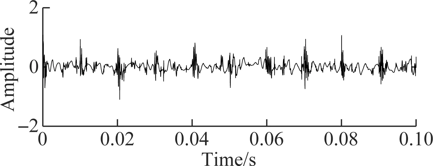
In order to verify the superiority of the proposed TDSST method in the noise reduction of strong impact signals, TDSST, wavelet threshold noise reduction (WT) and wavelet denoising using neighbouring coefficients (WD-NeighCoeff) method are used to process the noisy signal in Fig.3, and then the time domain waveform of Fig.4 is obtained by the inverse transformation.
Fig.4(a) is the reconstructed waveform of TDSST,βis 0.8 and the maximum search stepTis 50. Fig.5 is a schematic diagram of the time-frequency threshold denoising process. It can be found that the white noise is randomly distributed in the time-frequency spectrum. In the initial process of noise reduction, there are many noise points in the spectrum, and the noise part plays a significant role. As the threshold increases slowly, the noise part is filtered, and the difference between the adjacent spectra increases. Thus, the correlation coefficient of the time-frequency spectra shows a downward trend while the SNR increases and its curve shows an upward trend. Then, as the noise decreases, the main part of the signal becomes more and more prominent until the main part of the signal plays a greater role than the noise part. When the threshold continues to increase, the difference between adjacent spectra decreases instead and the correlation coefficient curve shows an upward trend. Due to the reduction of the noise, the SNR curve continues to rise. As shown in Fig.5, the correlation coefficient decreases first and then increases, while the SNR increases monotonously. When the noise part is basically filtered out, the main part of the signal begins to be filtered, and the curve of the SNR and the correlation coefficient reaches the peak simultaneously. Finally, as the main part of the signal is filtered, the difference between the adjacent spectra increases again, the correlation coefficient and SNR decrease simultaneously, and both curves show a downward trend. In practical applications, as the threshold increases continuously, fluctuations may occur during the decrementing of the posterior segment of the correlation coefficient curve. Therefore, the threshold corresponding to the first peak point after the first valley point on the curve is taken as the optimal noise reduction threshold, and the threshold corresponding to the peak point marked on the curve of correlation coefficient in Fig.5 is selected as the optimal threshold.
(b)
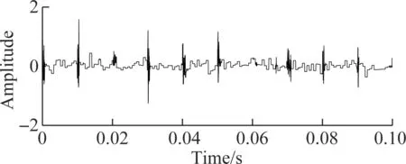
(c)Fig.4 Reconstructed waveform of bearing fault simulated signals using different denoising methods. (a) TDSST; (b) WT; (c) WD-NeighCoeff[14]
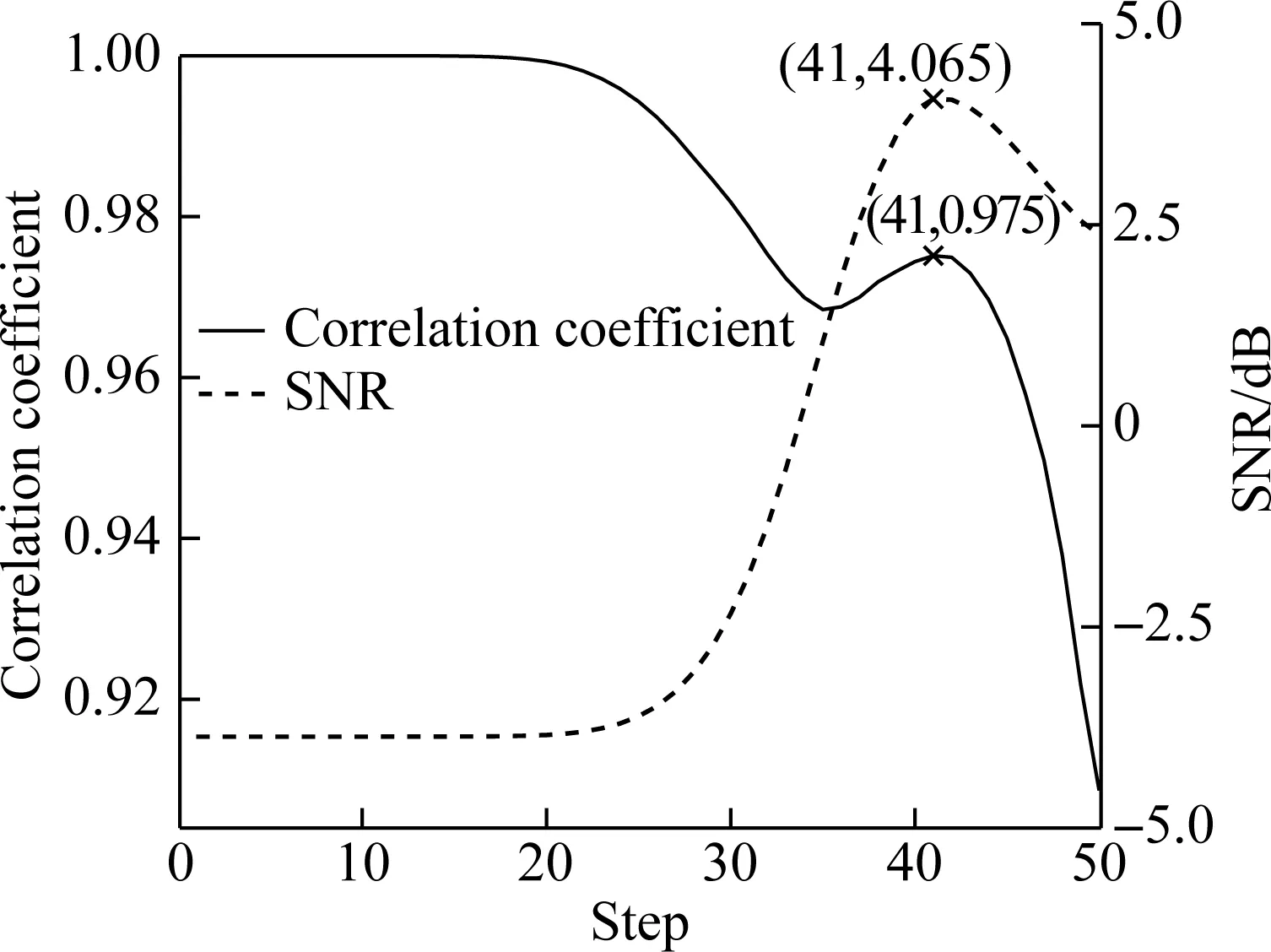
Fig.5 The schematic diagram of the time-frequency threshold denoising process
Fig.4(b) is the reconstructed waveform of WT, in which the sym5 wavelet function is selected, the number of decomposition layers is 4, and the soft threshold denoising method is adopted after testing. Fig.4(c) is the reconstructed waveform of WD-NeighCoeff, in which the sym8 wavelet function is selected and the number of decomposition layers is 4. By comparison, it is found that WT and the WD-NeighCoeff method have some denoising effect on the noisy signals with obvious impact components, but the period of the impact cannot be clearly identified in the reconstructed signal when the original SNR is low. The proposed method can obtain higher SNR. When the original SNR reaches -4 dB, the impact component with a period of 0.01 s can still be clearly found in the reconstructed signal, which proves that it is more suitable for the denoising of strong impact signals.
In order to further prove the superiority of the TDSST method, the signalx(k) shown in Eq.(13) is added with different degrees of noise, and then the above three methods are used for noise reduction and the SNR is calculated. The results shown in Tab.1 are the average values of 10 tests.

Tab.1 SNR of reconstructed signal dB
It is verified that the denoising effects of TDSST are better than those of the other two methods with the background of strong noise and weak noise for strong impact signals.
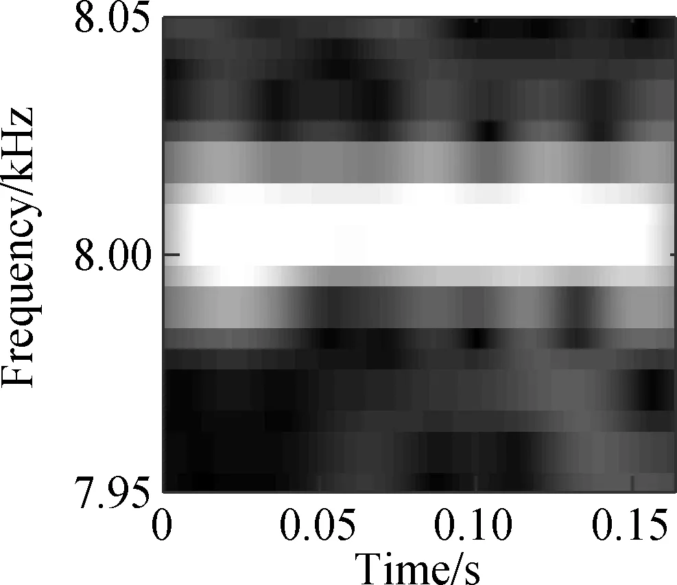
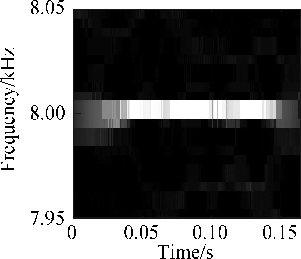
Then, in order to verify the superiority of TDSST in improving the time-frequency resolution, the signal in Fig.3 is processed by STFT, FSST and TDSST, respectively. The 8 000 Hz frequency component is amplified to obtain a local time-frequency diagram as shown in Fig.6. Fig.6(a) is the local time-frequency diagram obtained by the STFT. The time-frequency energy is relatively scattered, and due to the influence of strong noise, there are randomly distributed noises in addition to the 8 000 Hz frequency component. Fig.6(b) is the result of the FSST. Its resolution is significantly improved compared to Fig.6(a), and the energy is mainly concentrated near 8 000 Hz, but the noise part is also distributed on the diagram after being compressed. Fig.6(c) shows the results of the TDSST. It can be seen that the noise part is obviously reduced and the energy is concentrated at 8 000 Hz, and thus the time-frequency resolution is significantly improved. In order to accurately compare the effects of each method, the Rényi entropyRis used to measure the time-frequency resolution[15]: the Rényi entropy, the higher the time-frequency resolution will be. The Rényi entropy is calculated for the global time-frequency spectrum corresponding to the three pictures in Fig.6, which are 22.314, 20.459 and 18.245, respectively. The Rényi entropy of the time-frequency diagram obtained by the TDSST method is the smallest, which represents the highest time-frequency resolution, thus verifying the superiority of the TDSST method in improving the time-frequency resolution.
(14)
whereαgenerally takes 3, and the smaller the value of the Rényi entropy the higher the time-frequency resolution will be. The Rényi entropy is calculated for the global time-frequency spectrum corresponding to the three pictures in Fig. 6 which are 22. 314 20. 459 and 18. 245 respectively. The Rényi entropy of the time-frequency diagram obtained by the TDSST method is the smallest which represents the highest time-frequency resolution thus verifying the superiority of the TDSST method in improving the time-frequency resolution.
(a)
(b)

(c)
Fig.6 Local time-frequency diagrams. (a) STFT; (b) FSST; (c) TDSST
2 Fault Diagnosis Method of Rolling Bearing Based on TDSST and CNN
CNN is a deep learning network for identifying two-dimensional feature maps[16]. It can automatically extract features for classification from two-dimensional maps, which is similar to the processing of human brain vision systems. CNN contains multiple hidden layers, which can transfer features layer by layer and transform low-level features to high-level features to achieve feature learning and expression[17]. CNN is generally composed of convolutional layers, sampling layers and fully connected layers. The weight sharing attribute and the dimensionality reduction of the sampling layer greatly reduce the parameters that CNN needs to train, thus simplifying the network model and improving the training efficiency.
TDSST is used for the processing of CNN input data, and a fault diagnosis method for rolling bearings based on the TDSST and CNN is proposed. As shown in Fig.7, firstly, the rolling bearing vibration signal is processed by the TDSST, then the data set is divided into training set and test set; the CNN diagnosis model is obtained by training network with training set, and finally the test set is inputted into the model to obtain classification accuracy.
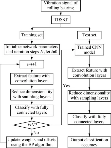
Fig.7 Fault diagnosis flowchart based on TDSST and CNN
3 Experiment Analysis
3.1 Data analysis
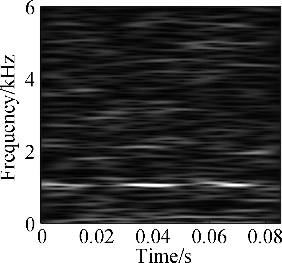
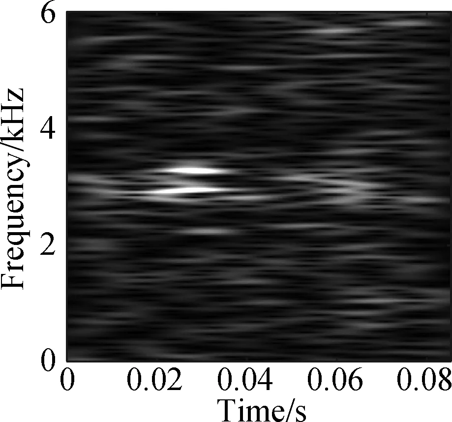
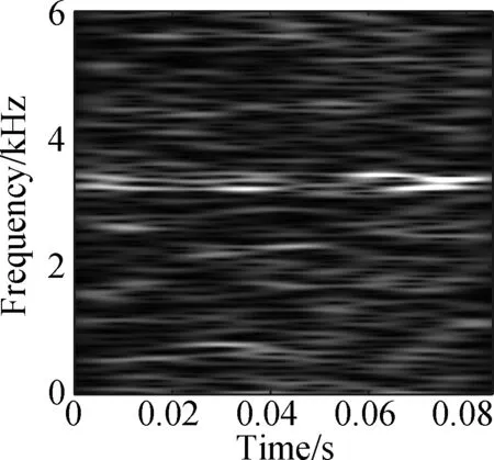
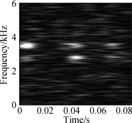
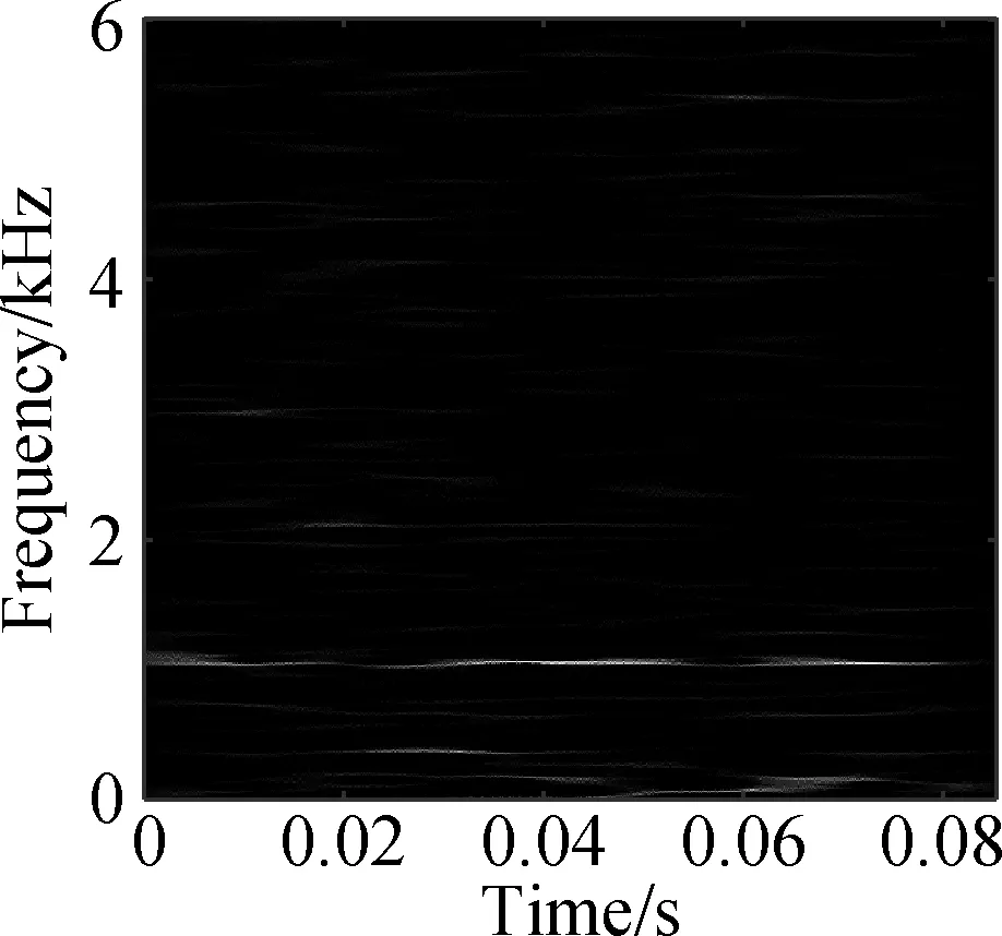
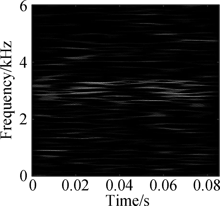
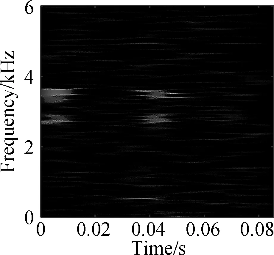
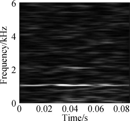
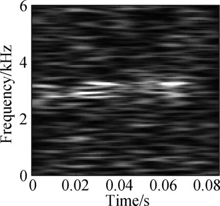
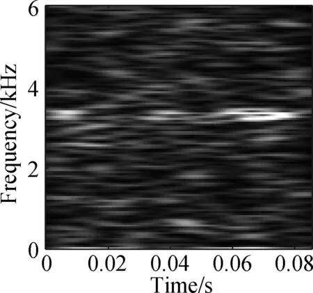
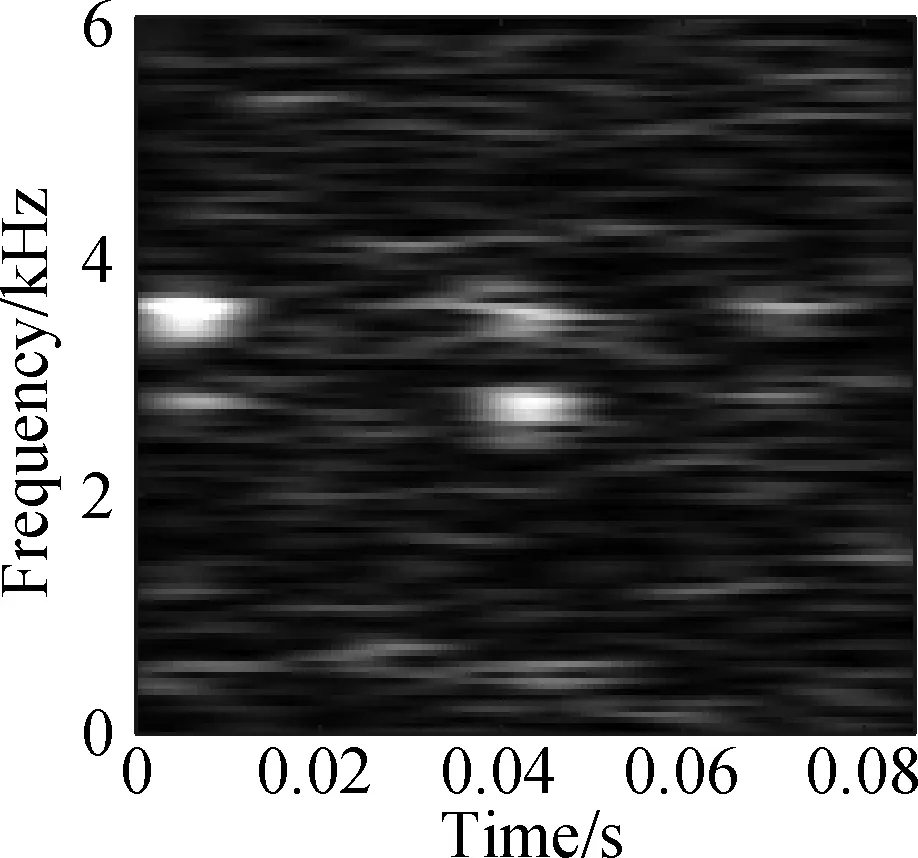
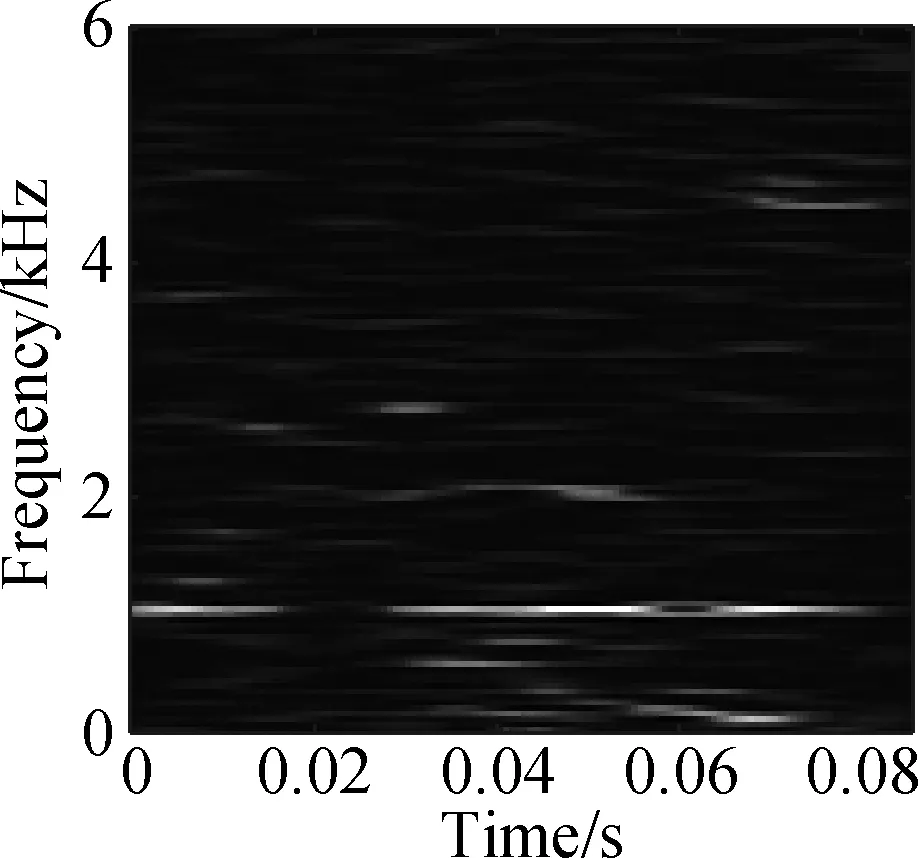
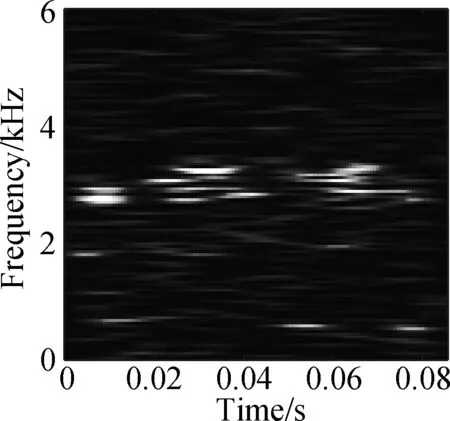
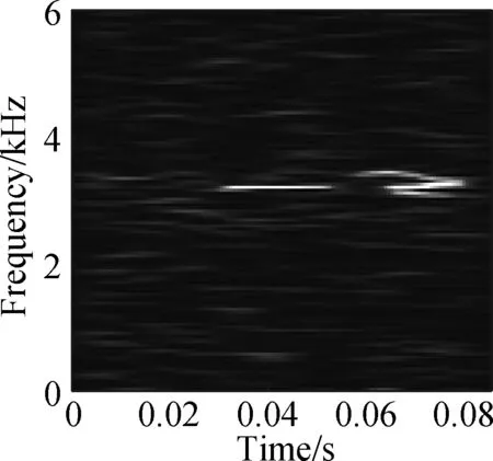
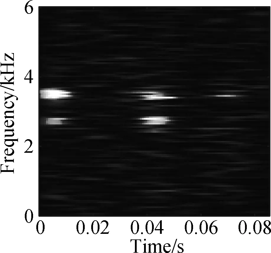
The open data set of the Case Western Reserve University is selected as the experimental data. The experiment simulates different degrees of inner ring faults, outer ring faults and rolling element faults by engraving the scratches of different depths on the inner ring, outer ring and rolling elements of the bearing. Faults with a depth of 0.177 8, 0.355 6, and 0.533 4 mm can be considered as minor, moderate, and severe faults, respectively. In this paper, the vibration data at 1 797 r/min is divided into 10 categories: normal condition, minor, moderate and severe inner ring faults, minor, moderate and severe outer ring faults and minor, moderate and severe rolling element faults. Each category selects 100 training data and 100 test data. The length of each sample data is 1 024, and the time-frequency diagram is converted to grayscale and compressed to 128×128 after processing with time-frequency analysis methods. Fig.8 and Fig.9 are the time-frequency diagrams of the normal condition, severe inner ring fault, severe outer ring fault and severe rolling element fault processed by the STFT and TDSST, respectively, under the condition of -4 dB. The noise part in Fig.8 is obvious, the main part of the signal is almost covered up, while the noise part in Fig.9 is mostly filtered out and the main part of the signal can be clearly seen after the TDSST.
(a)
(b)
(c)
(d)
Fig.8 STFT time-frequency diagram of a bearing in different states. (a) Normal condition; (b) Severe inner ring fault; (c) Severe outer ring fault; (d) Severe rolling element fault
(a)
(b)

(c)
(d)
Fig.9 TDSST time-frequency diagram of a bearing in different states. (a) Normal condition; (b) Severe inner ring fault; (c) Severe outer ring fault; (d) Severe rolling element fault
The time-frequency diagrams in Fig.8 and Fig.9 are compressed to a size of 128×128 and the results are shown in Fig.10 and Fig.11, respectively. It can be seen that the compressed diagrams after TDSST processing are significantly clearer than the compressed diagrams after STFT processing. It can be expected that the reduction of noise influence and the improvement of resolution can effectively improve the classification accuracy of CNN.
(a)
(b)
(c)
(d)
Fig.10 STFT time-frequency compression diagram of a bearing in different states. (a) Normal condition; (b) Severe inner ring fault; (c) Severe outer ring fault; (d) Severe rolling element fault
(a)
(b)
(c)
(d)
Fig.11 TDSST time-frequency compression diagram of a bearing in different states. (a) Normal condition; (b) Severe inner ring fault; (c) Severe outer ring fault; (d) Severe rolling element fault
3.2 Selection of CNN structure
At present, there is no strict standard to measure the quality of CNN structure. This paper mainly examines the robustness of the proposed method while the choice of the CNN structure is not the focus. Therefore, the CNN shown in Fig.12 is selected as the test network after tests. It uses two convolution layers, two sampling layers and one fully connected layer. Dropout is used in the fully connected layer to prevent over-fitting, and softmax is selected as the classifier.

Fig.12 Structure diagram of CNN
In Tab.2, C denotes the convolutional layer, and P denotes the sampling layer. C1 uses four 5×5 size convolution kernels, C2 uses six 3×3 size convolution kernels. The sampling layer uses mean sampling. The area size is 2×2, the step size is 2, and the ReLU function is selected as the activation function.

Tab.2 Structural parameters of CNN
3.3 Robustness analysis
In order to verify the robustness of each time-frequency analysis method combined with CNN for noise, firstly, the data is processed by each method and the network is trained. Then, the test data is added with different degrees of noise and processed by the corresponding method to test the network. To better verify the effect of the method, a variety of methods are used for comparison. The results are shown in Tab.3 and Fig.13. The first method was proposed by Li et al.[9], STFT and CNN were combined for diagnose, and the effect of parameters on the results was analyzed. The second method was proposed by Yuan et al.[18], which used continuous wavelet transform (CWT) as the data processing method, combined with CNN for diagnosis. The latter three methods use the methods mentioned in the first section as the processing methods of data, in which WTSTFT represents wavelet threshold noise reduction + STFT, NCSTFT represents wavelet denoising using neighboring coefficients + STFT.
The accuracies of the networks trained with different input samples under different noise conditions are compared in Tab.3. The accuracy results are the average values of 10 tests and the standard deviation of the accuracy of each case is calculated. It can be found that the accuracies of the networks obtained by using STFT, CWT WTSTFT and NCSTFT as preprocessing methods are relatively high only when SNR is high, and the accuracies rapidly decrease when SNR reduces to 4 dB or less. More-over, the accuracies of the network with WTSTFT and NCSTFT are lower than those with STFT and CWT, which also accords with the results of Fig.4. Although WT and WD-NeighCoeff can improve the SNR to some extent, the problem of loss of impact components in the signal cannot be ignored. However, the diagnostic method based on TDSST and CNN in this paper is highly accurate whether the SNR is high or low, especially when the SNR reaches -4 dB. The accuracy of STFT and CWT is reduced to about 40%, while the accuracy of TDSST remains still above 80%.
In addition, under different noise levels, the standard deviation of each method is small, indicating that the stability of each method is good and the methods are feasible.

Tab.3 The accuracies of CNN with different time-frequency analysis methods %
The accuracy of the proposed method is the highest in particular. The accuracy curves of 10 trials’ diagnosis results via the proposed method and other four methods when the SNR is 4 dB are displayed in Fig.13. It can be found that the method proposed in this paper is very accurate, and the results of the 10 trials are relatively similar. The curve varies more gently with more stability than in the other four methods. The above analysis results verify the superiority of the proposed method and the robustness of the network against noise.
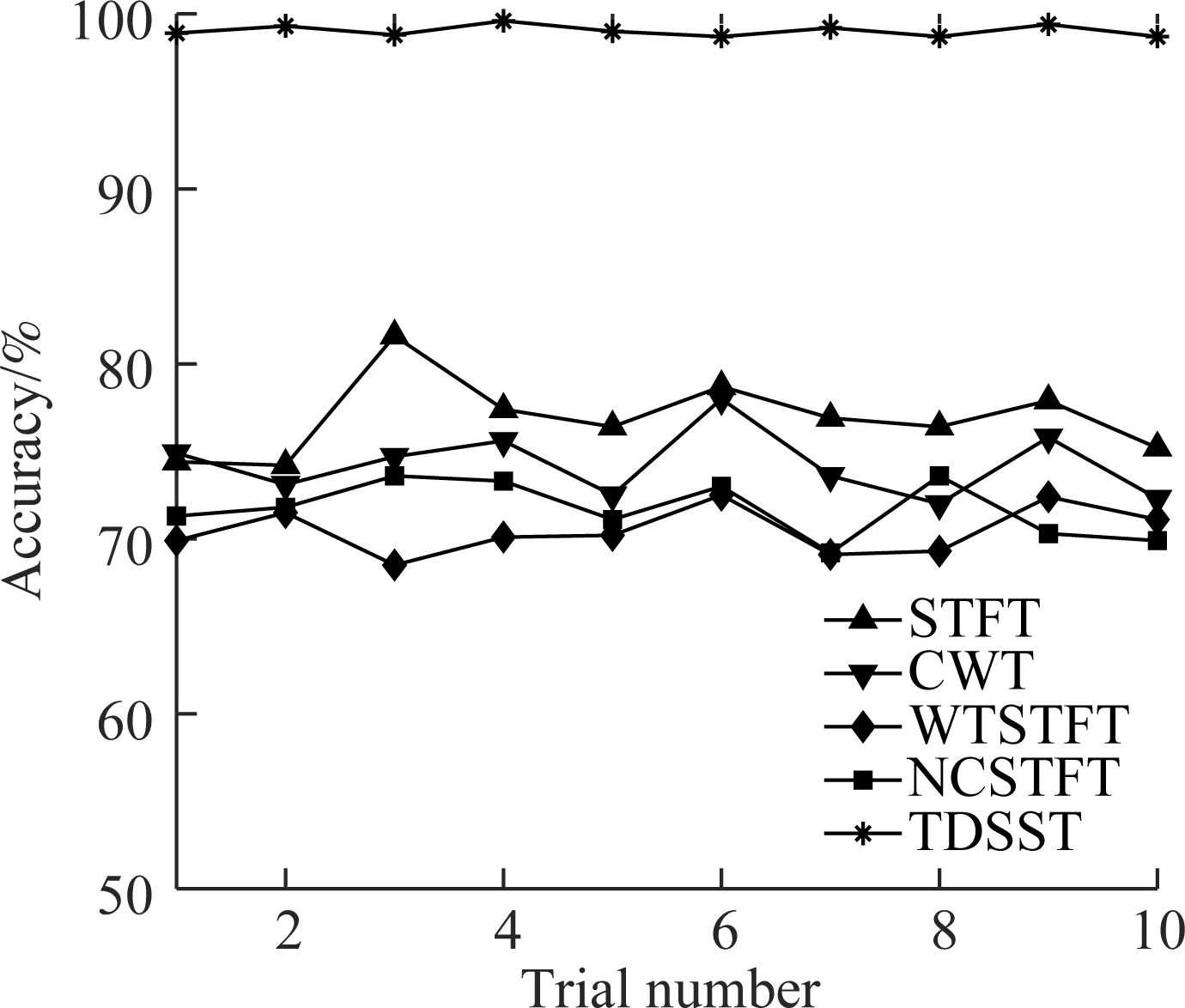
Fig.13 Diagnosis results of the 10 trials of four methods (Noise level is 4 dB)
4 Conclusions
1) Targeting the problem that it is difficult to determine the threshold by the traditional time-frequency threshold denoising method, a time-frequency threshold denoising method based on the threshold optimization via spectral correlation coefficient in STFT is proposed. The threshold can be increased in a variable length manner and determined according to the trend of the correlation coefficient curve. Then, the method is combined with synchrosqueezing transform, and a time-frequency analysis method based on TDSST is proposed. The superiority of the method in noise reduction and time-frequency resolution improvement is verified by simulation.
2) Targeting the problem that the working condition of the rolling bearing has strong noise and affects the judgment for the rolling bearing condition, a fault diagnosis method based on TDSST and CNN is proposed.
3) The rolling bearing fault diagnosis method based on TDSST and CNN is applied to the open bearing data of the Case Western Reserve University. The data set is divided into training set and test set. TDSST processing is applied to the training set, and the test set is added with different degrees of noise and processed by TDSST. Finally, the trained CNN network is used for diagnosis. By comparison, this method can effectively improve the diagnostic accuracy and has good robustness.
杂志排行
Journal of Southeast University(English Edition)的其它文章
- Effects of curing age on compressive and tensile stress-strain behaviors of ecological high ductility cementitious composites
- The cause of human fatigue and scenario analysisin the process of marine transportation
- An explicit representation and computation for the outer inverse
- Dispersion of graphene in silane coupling agent aqueous solutions
- Revenue optimization strategy of V2G based on evolutionary game
- Evaluation of rutting and low-temperature cracking resistancesof warm-mix recycled asphalt bindersunder the secondary aging condition
