OPTIMAL DIVIDEND-PENALTY STRATEGIES FOR INSURANCE RISK MODELS WITH SURPLUS-DEPENDENT PREMIUMS∗
2020-04-27JingweiLI李静伟
Jingwei LI(李静伟)
School of Economics and Management,Hebei University of Technology,Tianjin 300401,China
E-mail:jingweilicn@Yahoo.com
Guoxin LIU(刘国欣)
Department of Applied Mathematics and Physics,Shijiazhuang Tiedao University,Shijiazhuang 050043,China
E-mail:liugx@stdu.edu.cn
Jinyan ZHAO(赵锦艳)†
School of Science,Hebei University of Technology,Tianjin 300401,China
E-mail:zhaojinyan@hebut.edu.cn
Abstract This paper concerns an optimal dividend-penalty problem for the risk models with surplus-dependent premiums.The objective is to maximize the difference of the expected cumulative discounted dividend payments received until the moment of ruin and a discounted penalty payment taken at the moment of ruin.Since the value function may be not smooth enough to be the classical solution of the HJB equation,the viscosity solution is involved.The optimal value function can be characterized as the smallest viscosity supersolution of the HJB equation and the optimal dividend-penalty strategy has a band structure.Finally,some numerical examples with gamma distribution for the claims are analyzed.
Key words band strategy;risk models with surplus-dependent premiums;HJB equation;viscosity solution;Gerber-shiu function
1 Introduction
The surplus level X of an insurance company can be described by
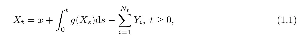
where x≥0 is the initial surplus;g is a premium function;Ntis a Poisson process with intensity λ >0;{Yi}i∈Nis a sequence of independent and identically distributed positive random variables with common distribution function Q,and assumed to be independent of Nt.Let function φx(t)be a solution of

for all x ≥ 0,t≥ 0.Note that φx(t)describes a deterministic trajectory of X between any two adjacent claim arrival epochs.Assume that the function g is positive,monotone,locally Lipschitz continuous and satis fies the following “speed condition”:

for some constants a≥0,b≥0.
To take into account the “severity”of ruin,we consider the so-called Gerber-shiu penalty function

where ω(x,y)is a function de fined on[0,∞)×(0,∞)representing penalty at ruin and satisfying the integrability condition

De fine the function(x,y)as

Hence,(1.4)can be written as

To give the rigorous formulation of the optimization problem,we de fine Ω as the set of paths with left and right limits,let(Ω,F,(Ft)t≥0,P)be the complete probability space generated by the process Xt.
A dividend strategy is a process L={Lt,t≥0},where Ltis the cumulative dividends of the company has paid out up to the time t.Given a dividend strategy L,the associated controlled surplus process XLis given by

The corresponding ruin time is denoted by

Note that unless it is necessary we will write τ instead of τLto simplify the notation.
We say that a dividend strategy is admissible if
•Ltis c`agl`ad(left continuous with right limits),nondecreasing,adapted with respect to the fi ltration(Ft)t≥0with L0=0;
•for any 0≤t<τ,the process Ltsatis fies

Denote by Πxthe set of all the admissible dividend strategies with initial surplus x ≥ 0.
Note that the controlled risk processis of finite variation,and,where−can only be positive at the arrival of the claims and−is positive only at the discontinuities of Lt.
We de fine the function VL(x)as the difference of the expected cumulative discounted dividend and the expected discounted penalty at ruin.We can write VL(x)as

where δ≥ 0 is the discount rate.The value function is de fined as

Optimal dividend problems of form(1.10)are a classical topic in stochastic control theory(see for instance Schmidli[13]).It was first shown in Gerber[10]by a discrete approximation and then a limiting argument that the optimal dividend strategy has a band type.This result was rederived by means of viscosity theory in Azcue and Muler[3].Moreover,they presented a very clear description of the band structure for optimal strategies and gave the first example with the optimal dividend strategy of two-band(see also Azcue and Muler[4]).Albrecher and Thonhauser[1]studied the dividend optimization problem for a risk process under force of interest.The same problem for a generalized risk model with investment incomes and debit interest was considered in Zhu[16].All of them show that the optimal dividend strategy is of band type as well.
A more general risk model with surplus-dependent premiums was proposed by Cai et al.[6],where they called them piecewise-deterministic compound Poission risk models.This risk model include many risk models as special cases,such as
•(Cram´er-Lundberg model) Premium flows in a constant rate c per unit time,i.e.,g(x)=c,x ≥ 0.Hence φx(t)=x+ct,t≥ 0.
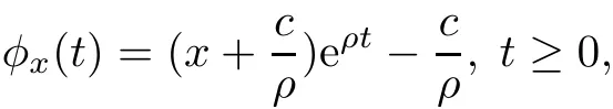
•(Constant interest model) All positive surplus earns interest at the constant rate ρ>0,i.e.,g(x)=ρx+c,x≥0.Hence
•(Credit interest and debit interest model) The positive surplus earns interest at rate ρ>0 while the negative surplus pays interest at a borrowing rate r>0,the function

Hence,for x≥0,

where t0=ln().
•(Regressive growth model) The surplus growth rate tends to regress to a mean premium rate c0>0 according to dg(x)=b0(c0−g(x))dx with g(0)=a0+c0and a0,b0>0.Hence,g(x)=+c0and
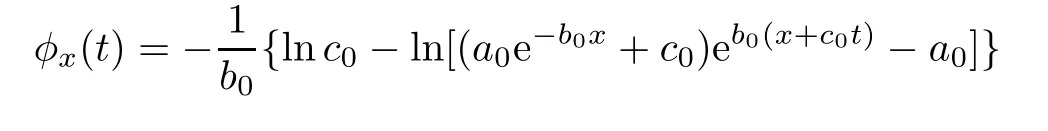
for t≥0.
Feng et al.[8]investigated the dividend problem for this model,especially for the cases with exponential claims.Marciniak and Palmowski[12]also studied the optimal dividend problem for this model and they firstly found the necessary and sufficient conditions for optimality of a single dividend-band strategy.
Recently,several alternative objectives were proposed,involving the expected discounted penalty at ruin,also called the Gerber-Shiu function.Liu et al.[17]studied the expected discounted fenalty function in a Markov-dependent risk model with constant dividend barrier and obtained the explicit formulas of Gorber-Shiu functions.Thonhauser and Albrecher[14]considered the dividend-penalty problem for the di ff usion model and the Cram´er-Lundberg model respectively,in which the penalty at the time of ruin is a given constant.They showed that the penalty can be used for balancing between pro fi t and safety in the portfolio.Avram et al.[2]studied the same problem for the spectrally negative L´evy process,in which the penalty payment at the moment of ruin is supposed to be an increasing function of the size of the de fi cit of ruin.Compared to the classical expected discounted dividend problem,the additional term re fined optimization criteria in the corresponding optimal control problems.Concerning the optimal dividend problem in the literature,the additional term is mostly in the cases,at which the penalty depends only on the de fi cit at ruin(see[7,11,12,15]etc.).The Gerber-Shiu function,in general,depends on the time of ruin,the surplus immediately before ruin and the de fi cit at ruin.We prefer a general Gerber-Shiu function as the additional term for the purpose of generality.
In this paper,we consider the dividend-penalty problem for the risk model with surplusdependent premiums.A salient feature of our model is the generality of pure jump models.We discuss the penalty function depend both on the surplus immediately before ruin and the de fi cit at ruin.Using the theory of viscosity solution,we show that the value function is the smallest viscosity supersolution of the HJB equation.The optimal dividend-penalty strategies have a band structure.This means that the payment of dividends depends only on the current surplus and it is characterized by three sets A,B and C which partitioned the state space of the surplus process.If the current surplus is in A,all the premium incoming is paid as dividends;if the current surplus is in B,a positive amount of money is paid as dividends in order to bring the surplus process back to A;and fi nally if the surplus is in C no dividends are paid.Moreover,The set A,B and C are proved to be closed,left-open and right-open respectively.Finally,a speci fi c algorithm is given and a new example for the constant interest model with gamma distribution for the claims is presented.In addition,we numerically analyze the e ff ect of the penalty for the three special cases of the risk model with surplus-dependent premiums:the Cram´er-Lundberg model,the constant interest model and the regressive growth model.It can be seen that the choice of different penalty function a ff ects the form of the optimal dividend strategy.As the penalty increases,a two-band optimal strategy may change to be a single-band one.
This paper is organized as follows.Some basic properties of the value function are studied in Section 2.Section 3 introduces the notion of viscosity solution and show that the value function is the viscosity solution of the HJB equation.The value function is characterized as the smallest viscosity supersolution of the HJB equation in Section 4.In Section 5,we show the existence of the optimal dividend-penalty strategy with a band structure.An algorithm of optimal n-band strategy is presented.Some numerical examples with gamma distribution for the claims show that different penalty functions a ff ect the form of optimal dividend strategy in Section 6.A conclusion is followed in Section 7.
2 Basic Properties of the Value Function
In this section,we show that the value function V introduced in(1.10)is well de fined and describe some of its properties.
Theorem 2.1The value function V(x)is well de fined and satis fies

for x≥0.
ProofIf g(x)is increasing,for any admissible dividend strategy L∈Πx,we haveand

If g(x)is decreasing,g(x)≤g(0)for any x≥0,we get
Give an initial surplus x≥0,consider the admissible dividend strategy L0∈Πxwhich pays x as a lump sum and then pays all the premiums incoming as dividend until the first claim,which in this strategy means ruin.More preciselyand by(1.5),we have

where τ1is the first claim time.By(1.10)we get the result.
Theorem 2.2The value function V is increasing,locally Lipschitz continuous and satisfies

for all b≥y>x≥0.
ProofGiven ε>0,take an admissible dividend strategy∈Πxsuch that(x)≥V(x)−ε.For each y>x≥0,we de fine a new strategy∈Πyas follows:pay immediately y−x as dividends and then follow the strategy¯L.The strategyis admissible and we have V(y)≥(y)=y−x+(x)≥y−x+V(x)−ε.
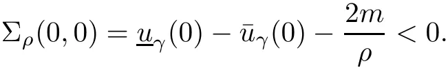
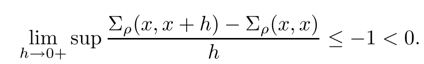
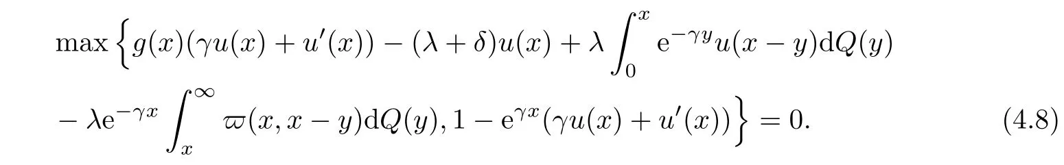
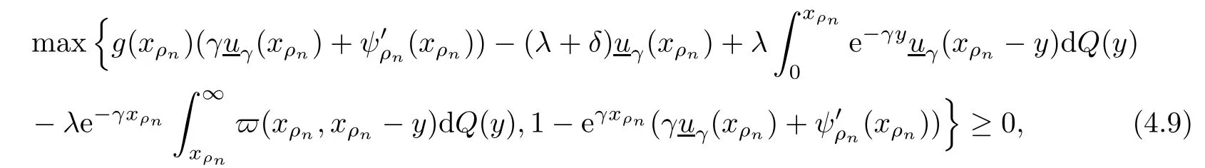
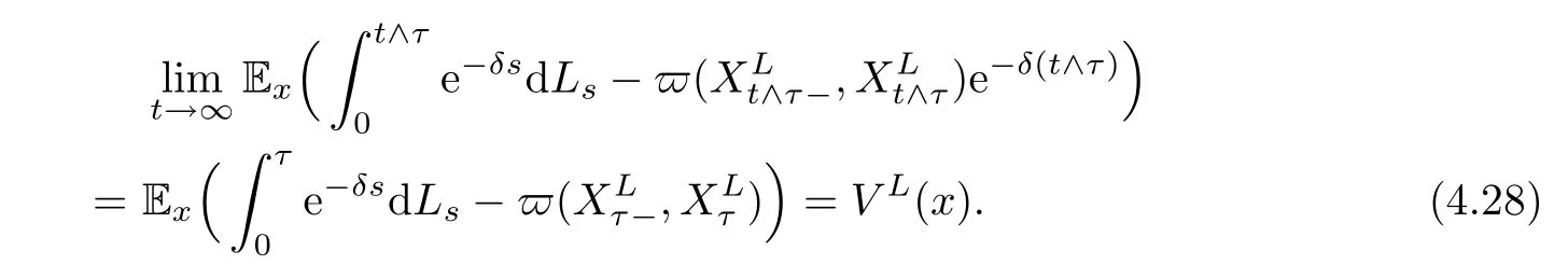
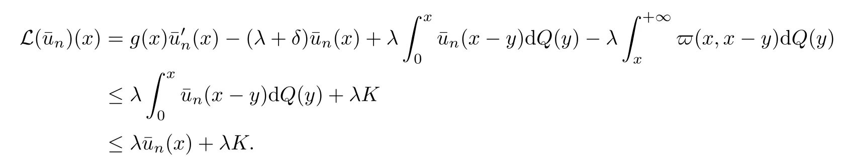
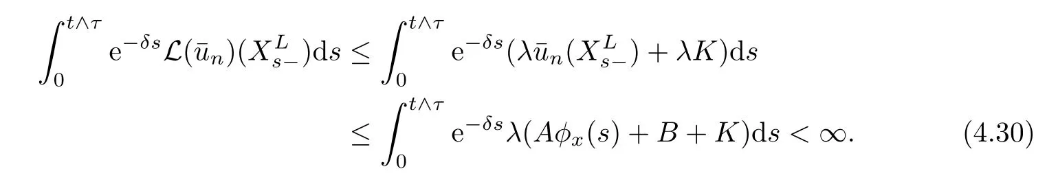
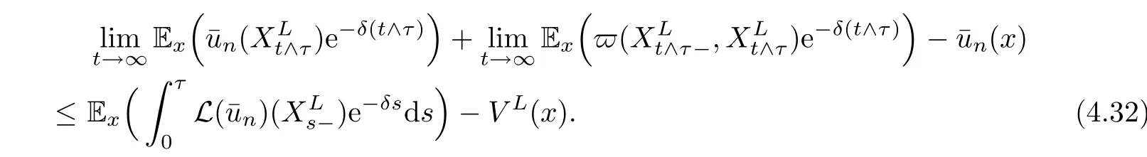
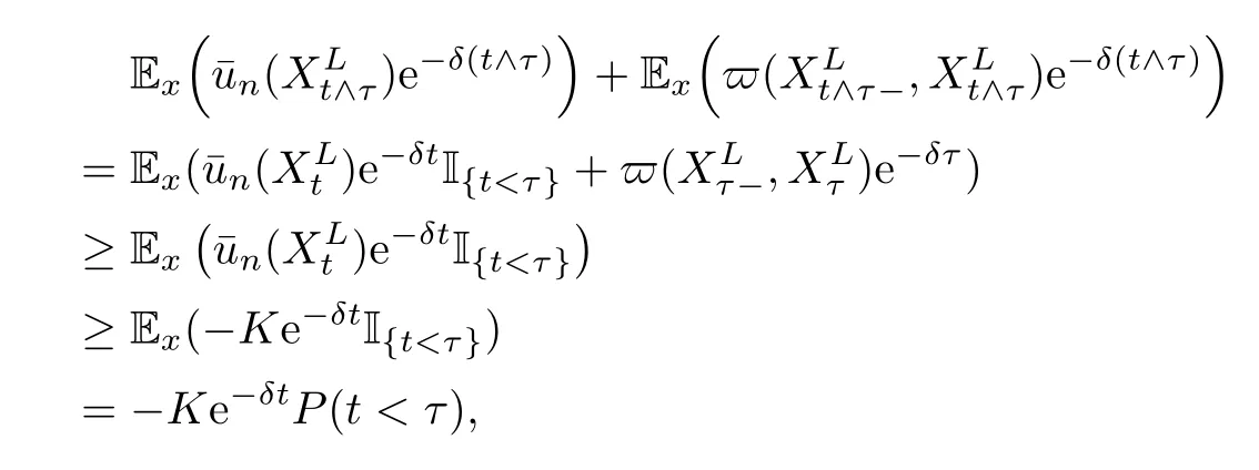
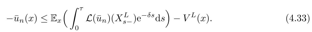
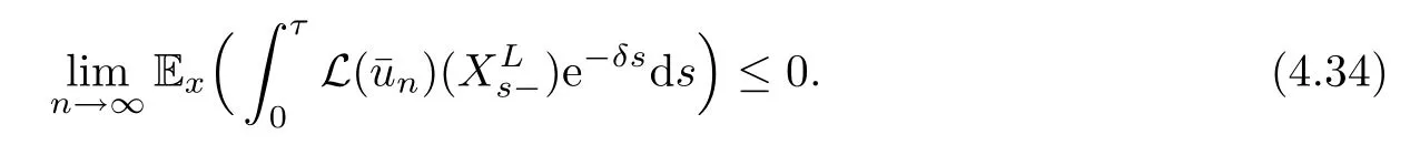
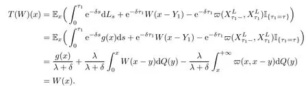
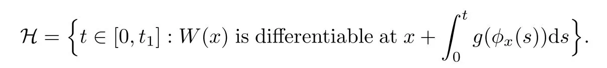
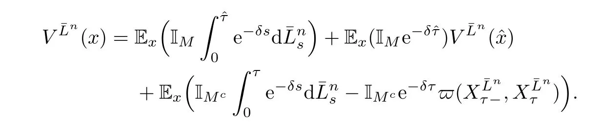
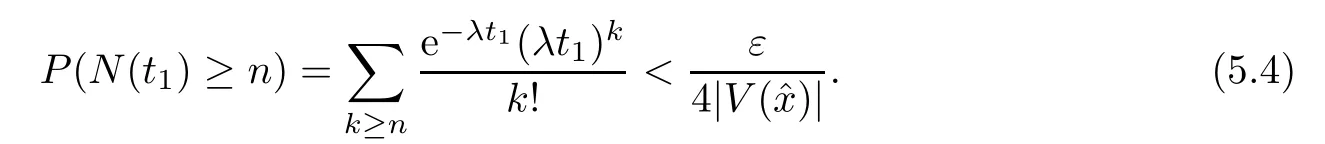
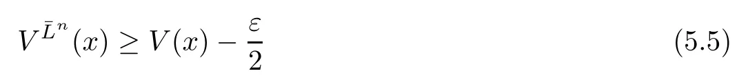
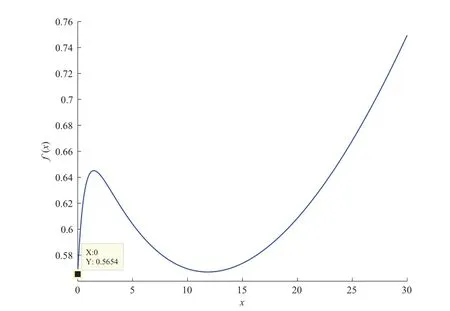
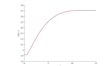
Given initial surplus y>x≥0 and ε>0,take an admissible dividend strategy∈Πysuch that(y)>V(y)−ε.Take the strategy L0∈Πxwhich,starting with surplus x,pay no dividends if Since the probability of reaching y before the arrival of the first claim is e−λt0,we get Then we obtain Applying standard arguments from stochastic control theory(e.g.Fleming and Soner[9])or an approach similar to that in Azcue and Muler[4],we get that the value function V ful fi lls the dynamic programming principle for any x≥0 and any stopping time.The HJB equation is where De finition 3.1A function:[0,∞)→R is a viscosity subsolution of(3.2)at x∈R+if it is locally Lipschitz continuous and any continuously differentiable function ψ :[0,∞)→ R with ψ(x)=and such that−ψ reaches the maximum at x satis fies max{L(ψ)(x),1−ψ′(x)} ≥0. If a function u:[0,∞)→ R is both a subsolution and a supersolution at x∈R+,it is called a viscosity solution of(3.2)at x. Remark 3.2At some points later on we will also make use of a different but equivalent de finition of viscosity subsolution and supersolution(see[5]).De fine a modi fied operator Lemma 3.3Let XLbe the controlled surplus process with initial value x>0,and u be a nonnegative continuously differentiable function in R+,then we can write for any finite stopping time τ∗≤ τ,where is a martingale with zero expectation. ProofSince Ltis nondecreasing and left continuous,it can be written as is a martingale with zero expectation becausefor s ≤ t and In the next theorem,we show that the value function V is a viscosity solution to equation(3.2).The supersolution proof is in the spirit of Azcue and Muler[4],whereas the approach of the subsolution proof is similar to Albrecher and Thonhauser[1]. Theorem 3.4The value function V(x)is a viscosity solution of(3.2)at any x>0. ProofLet us first prove that V(x)is a viscosity supersolution of(3.2).Given an initial surplus x0>0 and any l≥0,let us consider the admissible dividend strategy which pays dividend at constant rate l,that is.Let ϕ be a test function for supersolution of(3.2)at x0.From(3.1)for any t>0,we get So we have Inequality holds L(ϕ)(x0)≤ 0 for l=0,and 1−ϕ′(x0)≤ 0 for a large enough l>0.Therefore we obtain By De finition 3.1,V(x)satis fies the de finition of a viscosity supersolution. Next,we will show that V(x)is a viscosity subsolution of(3.2).Let ψ be a test function for subsolution of(3.2)at x0∈ (0,∞),we have max{L(ψ)(x0),1−ψ′(x0)} ≥ 0.We employ the proof by contradiction.Because ψ(x),ψ′(x)and V(x)are continuous,the operator L(ψ)(x)is continuous,too.There exist some h>0 and ς>0 such that for all x∈(x0−h,x0+h)=B and such that forˆx=x0±h,we have ψ(ˆx)−V(ˆx)>ς.Further choose h such that(x0−h,x0+h)⊂ (0,∞).Let{xn}n∈Nbe a sequence with xn→ x0and without loss of generality assume xn∈ B for all n ∈ N.Since V(x)and ψ(x)continuous,we have|V(xn)−ψ(xn)|→ 0.Next we look at the reserve with initial capital xn.De fine and denote by τ∗= τn∧ T for some T>0. Look at the set{τ∗= τn} first,we have that either x0+h is reached which implies,or a jump happens leading toandBecause V(x)is increasing and ψ(x)is increasing on B,we get We have from Lemma 3.3 and ψ′(x) ≥ 1 that Using(3.4)and(3.5)we obtain where βn= ψ(xn) − V(xn)converges to zero. Choose n large enough such that βn≤Then Following from(3.1)leads to the following contradiction If τ∗=0 which is only possible if τ∗= τn,then for the second term above The following comparison principle allows us to decide whether a viscosity supersolution dominates another viscosity subsolution by looking at their initial value.Since every viscosity solution is both a subsolution and supersolution,this will imply uniqueness for a given initial value.Actually in our situation,we have to modify the proof presented by Azcue and Muler[4].Although quite technical,the arguments are based on an appropriate combination of standard arguments from viscosity theory. De finition 4.1A continuous function u(x)has growth condition B1 if there exist some constants A≥1,B≥0 such that u(x)≤Ax+B for all x∈R+. Theorem 4.2Letandbe a subsolution and a supersolution of(3.2)for all x>0,respectively,both nondecreasing and nonnegative with growth condition B1.If,thenin R+. ProofArguing by contradiction,we assume that there exists a point x0such that>.Let γ>0 be a constant and for all x≥0,consider the functions for all y>x≥0.If γ1>0 small enough,we get by continuity that(x0)>(x0)for all γ∈(0,γ1]and satis fiesDe fine the set H={(x,y):0≤x≤y}.Let for all y≥x≥0.Let us de fine We also de fine and(xρ,yρ)=argWe obtain which is positive for ρ large enough,leading to Using the inequality We obtain that As a result for all ρ>4m.We can find a sequence ρn→∞such that(xρn,yρn)→().From(4.5),we haveand this give¯x=¯y. We show that(xρ,yρ)/∈∂H.First we look at and For all x>0 On the other hand,we have which is negative for ρ large enough.Hence we have proved that Σρ(x,y)is not achieved maximum on the boundary of H.Now we introduce two functions It can be easily shown that ψρ(x)and ϕρ(y)are both continuously differentiable. Then ψρn(x)and ϕρn(y)are also both continuously differentiable.Furthermore,uγ(x)− ψρn(x)=Σρn(x,yρn)−Σρn(xρn,yρn)attains its maximum 0 at xρn,and(y)−ϕρn(y)=−Σρn(xρn,y)+Σρn(xρn,yρn)reaches its minimum 0 at yρn.By De finition 3.1,we can see that(x)and(x)are respectively viscosity subsolution and supersolution of the following equation Therefore,by De finition 3.1,we obtain and B1and B2represent the first term and second term in the curly brackets of(4.9),respectively.D1and D2represent the first term and second term in the curly brackets(4.10),respectively.Then,max{B1,B2}≥0≥max{D1,D2}.So at least one of the inequalities B1≥D1and B2≥D2holds. On the one hand,we assume that B2≥D2is true.Noticing that From the assume we have From(4.11)and(4.12)we get Let N1(ε)be a positive integer such that for all n≥N1(ε),ρn≥4m.Since,then from(4.13),we can see that for all n≥N1(ε).Now let(ρn)n∈Nsuch that(xρn,yρn)→()as ρn→∞and.There exists an integer N2(ε)such that for all n ≥ N2(ε), Then for n ≥ N2(ε),we have From(4.3),(4.14),(4.15)and(4.16),it follows that for anyand n≥max{N1(ε),N2(ε)}, which is a contradiction.So B2≥D2does not holds. On the other hand,we prove that B1≥D1is not true.From(4.11)we have for all γ ∈ (0,γ1].By choosingfrom(4.4)and(4.18),we get Corollary 4.3There is at most one viscosity solution of(3.2)with boundary condition u(0)=u0among all the functions that satisfy growth condition B1. Lemma 4.4Fix x0>0 and let¯u be a nonnegative supersolution of(3.2)satisfying the growth condition B1.We can find a sequence of positive functions:R+→R such that (e)There exists a sequence cnwithsuch that ProofLet φ0(x)be a nonnegative continuously function with support include in(0,1)such thatR(x)dx=1.We de fine:R+→R as the convolution which gives Thus Let us de fine the function for x∈[0,x0].From(4.21),there exists xn∈[x,x+]such that If g(x)is increasing,from(4.19)and(4.20),we have By(4.23)and(4.24),we obtain Taking and satisfying cnwithIf g(x)is decreasing,we get and Taking and satisfying cnwithSo we get the result. Theorem 4.5The value function V(x)is the smallest viscosity supersolution of(3.2)satisfying growth condition B1. ProofLet L∈Πxbe any admissible dividend strategy,de fine XLas the corresponding controlled risk process starting at x.The function(x)de fined in Lemma 4.4 are continuously differentiable and≥1.Using Lemma 3.3 we obtain Since Ltis increasing,using the monotone convergence theorem we get Using(4.20),we get Using the integration by parts,we have Using the bounded convergence theorem,we obtain From(4.27),(4.28)and(4.31),we get From(1.5),we have which gives Then we get We show next that Given any ε>0,we can find T such that From Lemma 4.4 we can find n0large enough such that for any n≥n0, From(4.35),(4.36)and using the bounded convergence theorem we get(4.34). Then from(4.32),(4.33)and(4.34),we obtainThereforeSince V(x)is a viscosity solution of(3.2),we get the result. Theorem 4.6Consider a family of admissible dividend strategiessuch that∈Πxfor any initial surplus x≥0.If the function(x)is a viscosity supersolution of(3.2),then(x)is the value function. ProofSince(x)≤V(x)for all x≥0,and V satis fies growth condition B1,thenalso satis fies growth condition B1.From Theorem 4.5,we get the result. In this section,we show that there exists an optimal dividend-penalty strategy and it is a band strategy.A band strategy is characterized by three sets A,B and C which partition the space of the surplus process.Each of these sets is associated with a certain payment scheme. De finition 5.1We say that P=(A,B,C)is a band partition if A,B and C are disjoint sets with R+=A∪B∪C,A is closed,bounded,and nonempty;B is left open;C is right open;the lower limit of any connected component of B belongs to A;and there exists b≥0 such that(b,∞)⊂ B. De finition 5.2Given a band partition P=(A,B,C)and an initial surplus x≥0,we de fine recursively the admissible dividend strategy L∈Πxas follows: (a)in the case that x∈A,then pay all the premiums incoming as dividends until the first claim arrival τ1.Afterwards,follow strategy corresponding to initial surplus x−Y1if x−Y1≥ 0,where Y1is the size of the first claim.If x− Y1<0 i.e.,τ1= τ,take the fi nal penalty at the time of ruin; (b)in the case that x∈B,there exists an open interval(x0,x1)⊂B with x0∈A;then pay x−x0as dividends instantly.Afterwards,follow the strategy corresponding to initial surplus x0∈A; (c)in the case that x∈C,there exists an open interval(x,x1)⊂C with x1∈A;take Lt=0 up to τcthe exit time of C.Afterwards,follow the strategy corresponding to initial surplus. Theorem 5.3Consider a band partition P=(A,B,C);any Borel-measurable function W(x)which is left continuous at the upper limit of the connected component of C,it is right continuous at lower limits of the connected components of B,it has derivative equal to 1 on B,it is an almost-everywhere solution of L(W)(x)=0 in the connected components of C,and it is a solution of Λ(W)(x)=0 in A,should be the function VP. ProofLet Π(P)={L ∈ Πxwith x ≥ 0}be the band strategy associated to the band partition P.Let us de fine the operator T on the set of Borel-measurable,and locally bounded function as The family Π(P)is called the band strategy associated to the band partition P. Let us consider the operator Λ de fined as where τ1and Y1are the time and size of the first claim respectively.Given an initial surplus x≥0,we have m(x)is finite because m(x)=x if x∈A∪B,and if x∈C,m(x)is the upper bound of the connected component of C.Given any M∈A∪B consider the complete metric space BM={W:[0,M]→R+}where BMis Borel-measurable and bounded,with the metricNote that for any x≤M,we have m(x)≤M and so T(W)(x)is well de fined and bounded in[0,M].On the other hand So T:BM→BMis a contraction operator with modulus<1 and therefore it has a unique fixed point.Since any connected component of C is bounded we have that if supA∪B=∞,then there exist a unique locally bounded function:R+→R with.We get that VPis the unique fixed point by T(VP)=VP.If x ∈ A,then Λ(W)(x)=0 and so If x∈B,x0=max{y If x∈C,consider x1=min{y>x and yC},x(t1)=φx(t1)=x1∈A and x(t)∈C for t∈[0,t1).The set de fined by Since x(t)is increasing,exist t1>0 such that x(t1)=x1∈A.Therefore The following two theorem can be shown by using a similar idea as in Albrecher and Thonhauser[1]and Azcue and Muler[3]. Theorem 5.4Let us de fine for anyˆx≥x,the set ProofAs a first step we show that for all n≥0.The proof is by induction on n.By de finition of V(x),(5.2)holds for n=0.Taking n≥1 and ε>0,we can findsuch thatWe will construct for anyan admissible dividend strategysuch thatWe now de fine the strategy:starting with x≤follow the strategywhile;if the surplusreaches,pay out the premiums incoming as dividends until the next claim,if Y is the size of this claim,follow the strategywith initial surplus−Y if−Y≥0;if−Y<0,the penalty is taken at the time of ruin.Note that the strategyis measurable. From the following two inequalities we get the required result.and,which gives Finally,given any ε>0 and x∈[0,],we can find an admissible dividend strategy∈Πx,ˆxsuch that V(x)−(x)<ε.Choose t1>0,satisfying Then for this fixed t1choose n≥1 large enough such that and N the set of all the paths with initial surplus x∈[0,]and τ∗finite.We de fine the dividend strategyas follows:for all t<τ∗and if t=τ∗pay outimmediately and then pay the premiums incoming as dividends until the arrival of the next claim.Sinceis admissible,it is easy to see thatis also admissible.We have Thus Theorem 5.5Let us de fine for anyˆx≥x,the set ProofGiven any ε>0,we will find an admissible dividend strategysuch that V(x)−(x)<ε for all x∈[0,].Let us de fine Consider and de fine Let us take an admissible dividend strategysuch that for all x∈ We de fine recursively strategiesas follows:k=0,;k>0,for initial reserve x≤xn0,follow the strategy¯L while.When the reservereaches,pay out immediately the differenceas dividends and then follow the strategywith initial reserve xn0.For initial reserve x∈(xn0,],pay out immediately the difference x−xn0as dividends and then follow the strategywith initial reserve xn0. As the first step,we show that V(x)−(x) If x∈[xn0,],from(5.9),(5.10),(5.11)and(5.12),we have If x∈[0,xn0),let M be the set of all the pathswith initial reserve x that reach xn0in finite time and let τxbe the first time that a path in M reaches xn0.We get From(5.12),we get So If x∈[0,xn0),let Θ be the set of all the paths with initial reserve x that reachin finite time and letbe the first time that a path in Θ reaches,we have From(5.13),(5.14)and(5.15),we obtain Note that the fastest way to arrive to reservefrom initial reserve xn0is by paying out no dividends.It will take at least a period time of t0to pass through the interval[xn0,],where t0satisfyingand xn0∈[0,].We get(g(0)∨g())t0.Let us de fine=inf{t>0:,then we have Let N be the set of all the pathswith initial reserve x whenis finite.We de fine the strategyas follows:for all t<,if t=τ,pay out immediatelyas dividends,and then pay out the premiums incoming as dividends up to the arrival of the next claim.Sinceis admissible,the strategyis also admissible.We have Therefore From(5.17)and(5.18),we get Lemma 5.6The function Λ(V)(x)is right continuous with possible upward jumps and satis fies Λ(V)(x)≤ 0 for all x ≥ 0. ProofSince V is locally Lipschitz continuous and it is a viscosity solution of(3.2),then it satis fies Since Q is right continuous with possible upward jumps,so is Λ(V)(x),then we have that Λ(V)(x)≤0 for all x≥0. Lemma 5.7Consider a point y≥0 where V(x)is differentiable,let us de fine the function Wy(x)=V(x)I{x≤y}+(V(y)+x−y)I{x>y}.Then (a)Wy(x)≤V(x). (b)If Wy(x)is a viscosity supersolution of(3.2)in(y,∞),then Wy(x)=V(x)in R+. Proof(a)Because Wy(0)=V(0)and Wy′(x)≤ V′(x)a.e.,we get the result. In order to prove(b)let us show that Wy(x)≥V(x).By Theorem 4.5,it is need to prove that Wy(x)is a viscosity supersolution of(3.2)at y.The righthand derivative in y is given throughThere exists an appropriate test function ψ(x)with the supersolution property if and only ifFrom the de finition Wy(y)=V(y)and the supersolution property of V(x)implies that In this case we get ψ′(y)=1 showing Wy(x)is a viscosity supersolution of(3.2).The proof of(c)is analogous to the proof of(a)but follows from Theorem 5.4 and Theorem 5.5. De finition 5.8Let us de fine P∗=(A∗,B∗,C∗)as • A∗={x∈ R+such that Λ(V)(x)=0}, • B∗={x ∈ (0,∞)such that V′(x)=1 and Λ(V)(x)<0}, • C∗=(A∗∪B∗)c. Inspired by Azcue and Muler[4],we give the following two theorems to verify P∗is a partition and VP∗=V. Theorem 5.9P∗is a band partition,which satis fies (a)A∗is closed. (b)B∗is left-open. (c)If(x0,x1]⊂B∗and x0/∈B∗then x0∈A∗. (d)C∗is right-open. (e)If 0≤a<1,there exist˜x such that(,∞)⊂B∗. Proof(a)From Lemma 5.6 we get A∗is closed. (b)Taking x∈B∗,and then by Lemma 5.6,there exists h>0 such thatforand V(x)is differentiable at x−h.Consider the function Wx−h(x)introduced in Lemma 5.7,we have thatandfor all Therefore Wx−h()is a supersolution of(3.2)in(x−h,x].By Lemma 5.7,we get Wx−h()=V()in(x−h,x]and then(x−h,x]⊂B∗. (c)Suppose that(0,x1)⊂ B∗,we are going to prove that 0∈ A∗.Consider the admissible dividend strategy∈Π0withup to the first claim τ1(where the ruin occurs),thenTake x ∈ (0,x1),V′(x)=1 by Theorem 5.5,we get Suppose that(x0,x1)⊂B∗with x0>0 and x0/∈B∗,we now show that x0∈A∗.If V′(x0)=1 then Λ(V)(x0)=0,therefore x0∈ A∗.We assume that this is not the case.If V′(x0)6=1,we have that and Then for any b with b∈(1,a],we have Then we have which implies Taking limits b→ 1 gives Λ(V)(x0)≥ 0.From Lemma 5.6 we obtain Λ(V)(x0)≤ 0,Therefore we get Λ(V)(x0)=0 and so x0∈ A∗. (d)Let us prove now that C∗is right open.Given x ∈ C∗,we have Λ(V)(x)<0 and so there exists ε>0 such that Λ(V)()<0 in(x,x+ε)and this implies that(x,x+ε)⊂C∗∪B∗.If there exists x1∈(x,x+ε)such that x1∈B∗,we can find x0∈A∗and x1with x≤x0 (e)To prove the result,we will show that if˜x is large enough,then W˜x(x)is a viscosity supersolution of(3.2)for all x∈(˜x,∞).Since(x)=1 in(˜x,∞),we only need to show L(W˜x)(x)≤0 in(,∞). Case 1If g(x)is decreasing,we have By Theorem 2.1,we get L(W˜x)(x)≤0 in(,∞)for all Case 2If g(x)is increasing,from(1.3),we get which gives g(x)≤ δ(ax+b). Theorem 5.10The band strategy Π(P∗)is optimal,that is V(x)=VP∗(x)for all x∈R+. ProofIt is enough to see that V(x)satis fies the conditions of Theorem 5.3 for the partition P∗={A∗,B∗,C∗}.By Theorem 2.2,V(x)is locally Lipschitz continuous,and by De finition 5.8,V′(x)=1 on B∗and Λ(V)(x)=0 on A∗.We have that V(x)is a viscosity solution of(3.2)and V′(x)>1 for x ∈ C∗where V(x)is differentiable,so V(x)is an almost everywhere solution of L(V)(x)=0 in the connected components of C∗. The algorithm is similar to Azcue and Muler[4]and Schmidli[13],which is not only suitable for the Cram´er-Lundberg model but also for surplus-dependent premiums risk models.We say that a band strategy is an n-band strategy if=n.We assume that n is finite.On[0,]we have to solve the equation W e consider the partition P1with barrier level a1first,and where f(x)is unique solution of(6.1)with f(0)=1,therefore,the minimum of f′(x)which is taken at x=.We check whether(x)is a viscosity solution of(3.2).If(x)ful fi lls(3.2)we are done,and if not we look for the best two-band partition.Given any pair of values b1 We consider the constant interest risk model,i.e.,g(x)=ax+c.Take a gamma claim-size distribution with Q(x)=1−(1+x)e−xand the parameters a=0.02,c=21.4,λ =10,δ=0.1. We take ω(x,y)=ker(y−x)with k=0.05 and r=.The optimal band partition is a two-band strategy with A∗={0,12.59},B∗=(0,0.50]∪(12.59,∞),C∗=(0.50,12.59).Figure 1 give f′(x)with f(0)=1,where f(x)is the solution to(6.1).It is easy to see that the minimum of the derivative is taken in zero.Thus,pay out all the premiums incoming at zero.The V(x)and V(x)−x are shown in Figure 2 and Figure 3 respectively. Figure 1 f′(x)with f(0)=1,where f(x)is the solution to(6.1) Figure 2 V(x)with gamma distribution for the constant interest model Figure 3 V(x)−x with gamma distribution for the constant interest model In addition,we analyze the e ff ect of the penalty for three special cases of the risk model with surplus-dependent premiums:the Cram´er-Lundberg model(i.e.,g(x)=c),the constant interest model(i.e.,g(x)=ax+c)and regressive growth model(i.e.,g(x)=a0e−b0x+c).We take a gamma claim-size distribution with Q(x)=1−(1+x)e−xand the parameters c=21.4,a=0.02,a0=2,b0=0.4,λ =10,δ=0.01.We also take ω(x,y)=.We consider the particular cases k ∈ {0,0.01,0.02,0.03,0.04,0.05,0.06,0.07,0.08,0.09}.For the Cram´er-Lundberg model,if k ∈ {0.08,0.09}the optimal strategy is a single-band strategy at level,while in other cases of k it is optimal to adopt a two-band strategy with=0.The bond levels of the optimal strategies are summarized in Table 1.The bond levels of the optimal strategies for the constant interest model and the regressive growth model are displayed in Table 2 and Table 3,respectively.In Table 1 and Table 2,the form of the optimal dividend strategy for k=0 can be found in Azcue and Muler[3]and Albrecher and Thonhauser[1],respectively. From Table 1,in the case of two-band strategy we observe that=0,decreases andincreases as k increases,while in the case of single-band strategy we find that(>0)increases as k increases.From Table 2 and Table 3,we find the similar conclusion. Table 1 The optimal band levels for the Cram´er-Lundberg model Table 2 The optimal band levels for the constant interest model Table 3 The optimal band levels for the regressive growth model We study the optimal dividend-penalty problem for the risk models with surplus-dependent premiums.The risk model with surplus-dependent premiums is the more general insurance risk model,which include many risk models as special cases,such as the Cram´er-Lundberg risk model,the constant interest risk model,the regressive growth risk model etc..We prove that the value function is the unique viscosity solution of the associated HJB equation and the optimal strategies have a band structure.We also give a speci fi c algorithm to calculate the optimal dividend strategy and present an example for the constant interest model with gamma distribution for the claims.In addition,we analyze the e ff ect of the penalty function on the three special cases of the risk model with surplus-dependent premiums:the Cram´er-Lundberg model,the constant interest model and the regressive growth model.With the penalty function increasing,the optimal band levels are also increasing.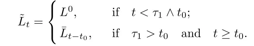


3 HJB Equation and Viscosity Solution


4 Characterization of the Value Function


5 Optimal Dividend-Penalty Strategy


6 Numerical Examples


7 Conclusion
杂志排行
Acta Mathematica Scientia(English Series)的其它文章
- HILBERT PROBLEM 15 AND NONSTANDARD ANALYSIS(I)∗
- INFINITELY MANY SOLITARY WAVES DUE TO THE SECOND-HARMONIC GENERATION IN QUADRATIC MEDIA∗
- COMPLEX SYMMETRIC TOEPLITZ OPERATORS ON THE UNIT POLYDISK AND THE UNIT BALL∗
- THE BOUNDEDNESS FOR COMMUTATORS OF ANISOTROPIC CALDER´ON-ZYGMUND OPERATORS∗
- GROUND STATES FOR FRACTIONAL SCHR¨ODINGER EQUATIONS WITH ELECTROMAGNETIC FIELDS AND CRITICAL GROWTH∗
- MULTIPLE JEEPS PROBLEM WITH CONTAINER RESTRICTION∗