Morphology Similarity Distance for Bearing Fault Diagnosis Based on Multi-Scale Permutation Entropy
2020-03-16JinbaoZhangYongqiangZhaoLingxianKongandMingLiu
Jinbao Zhang, Yongqiang Zhao, Lingxian Kong and Ming Liu
(School of Mechatronics Engineering, Harbin Institute of Technology, Harbin 150001, China)
Abstract: Bearings are crucial components in rotating machines, which have direct effects on industrial productivity and safety. To fast and accurately identify the operating condition of bearings, a novel method based on multi-scale permutation entropy (MPE) and morphology similarity distance (MSD) is proposed in this paper. Firstly, the MPE values of the original signals were calculated to characterize the complexity in different scales and they constructed feature vectors after normalization. Then, the MSD was employed to measure the distance among test samples from different fault types and the reference samples, and achieved classification with the minimum MSD. Finally, the proposed method was verified with two experiments concerning artificially seeded damage bearings and run-to-failure bearings, respectively. Different categories were considered for the two experiments and high classification accuracies were obtained. The experimental results indicate that the proposed method is effective and feasible in bearing fault diagnosis.
Keywords: bearing fault diagnosis; multi-scale permutation entropy; morphology similarity distance
1 Introduction
Rolling element bearings are critical components in rotating machines and their states in operation directly affect industrial productivity and workers’ safety. Fault diagnosis in the early stage could provide maintenance guidance and avoid huge economic losses so a fast and precise method is necessary. Traditionally, the framework of fault diagnosis for bearings consists of five parts: data acquisition, data preprocessing, feature extraction, dimensionality reduction, and fault classification[1-3].
Prominent features are critical in fault diagnosis, so multiple domain features have been investigated, including root mean square (RMS), kurtosis, and skewness in time domain and frequency domain, and short-time Fourier transform (STFT)[4]in time-frequency domain[5]. To deal with nonlinear dynamic characteristics of bearing fault signals, several entropy-based approaches have been proposed, such as approximate entropy (ApEn)[6-7], sample entropy (SaEn)[8-9], fuzzy entropy[10-11], multiscale entropy (MSE)[12-13], and permutation entropy (PE)[14-15]. PE can measure the complexity of time series through comparing adjacent values, which is simple, immune to noise, and suitable for online monitoring. Based on the PE method, multi-scale permutation entropy (MPE) was developed by Aziz and Arif[16]and was employed to estimate the complexity of the signals in different scales. MPE excels at its stability and robustness and performs better than PE in the application of bearing fault diagnosis[17-21].
Traditional approaches for dimensionality reduction are principal component analysis (PCA)[1]and modifications like locally linear embedding (LLE)[2],Laplacian score (LS)[3], and non-negative matrix factorization (NMF)[4]. With the selected features, the fault diagnosis should be performed with a classifier, which consists of two types based on the vibration data, i.e., statistical models[1,3]and data-driven models[2, 11, 13, 15, 20-22]. The two classifiers have their own advantages for bearing fault classification but are with deficiencies that they are complex and difficult to implement.
Since the essence of fault diagnosis is the problem of pattern recognition, distance would be an essential factor for the discrimination of different feature vectors. Hence, the nearest neighbor principle should be considered and the fault type could be identified with the smallest distance. For example, dynamic time wrapping[23]has been applied in bearing fault diagnosis[24], which measures the similarity of vectors with different length, but is with high computation complexity at the same time. In addition, not all the distances (e.g., the Euclidean distance) could differentiate the pattern. Based on the above analysis, MSD[25]is applied in this paper for bearing fault classification, which considers the shape of feature vectors and is simple to implement because no tuning parameters need to be set up or optimized compared with the abovementioned classifiers.
The rest of this paper is organized as follows: a brief review of the theoretical background concerning MPE and MSD is provided in Section 2; Section 3 illustrates the procedure of MPE-MSD, and two experiments considering different categories are designed and implemented to verify effectiveness of the proposed method in Section 4; finally, conclusions are drawn in Section 5.
2 Theoretical Background
2.1 Multi-scale Permutation Entropy
PE[14]was firstly used for detecting the dynamic change of time series data and to overcome former entropy method limitations such as the requirement of long datasets and high computational cost. The definition and implement procedure of PE are described as follows.
Considering a time series {x(k),k=1,2,…,N}, themdimensional vector at timeican thus be constructed as

i=1,2,…,N-(m-1)τ
(1)
x(i+r0τ)≤x(i+r1τ)≤…≤x(i+rm-1τ)
(2)
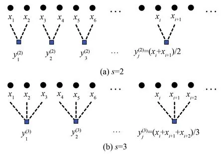
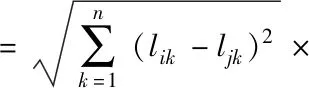
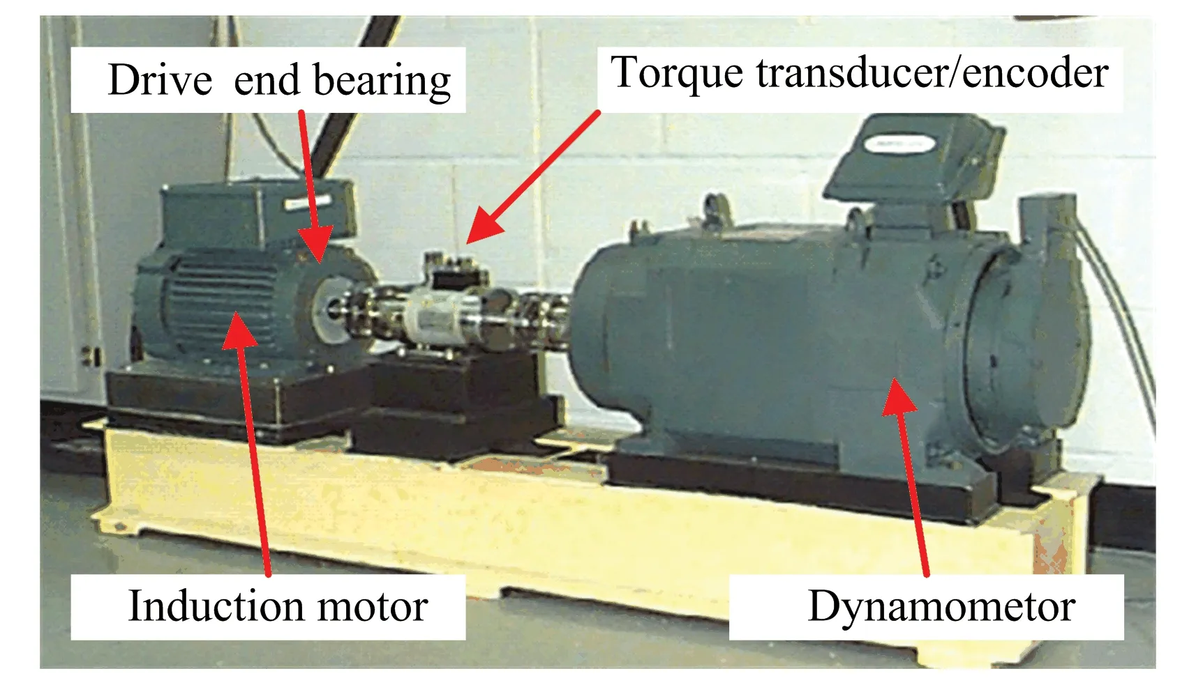
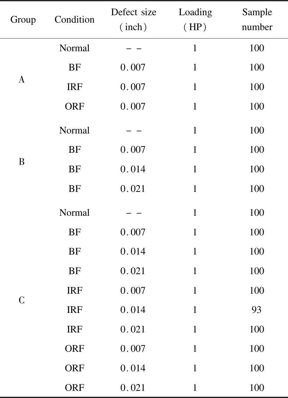
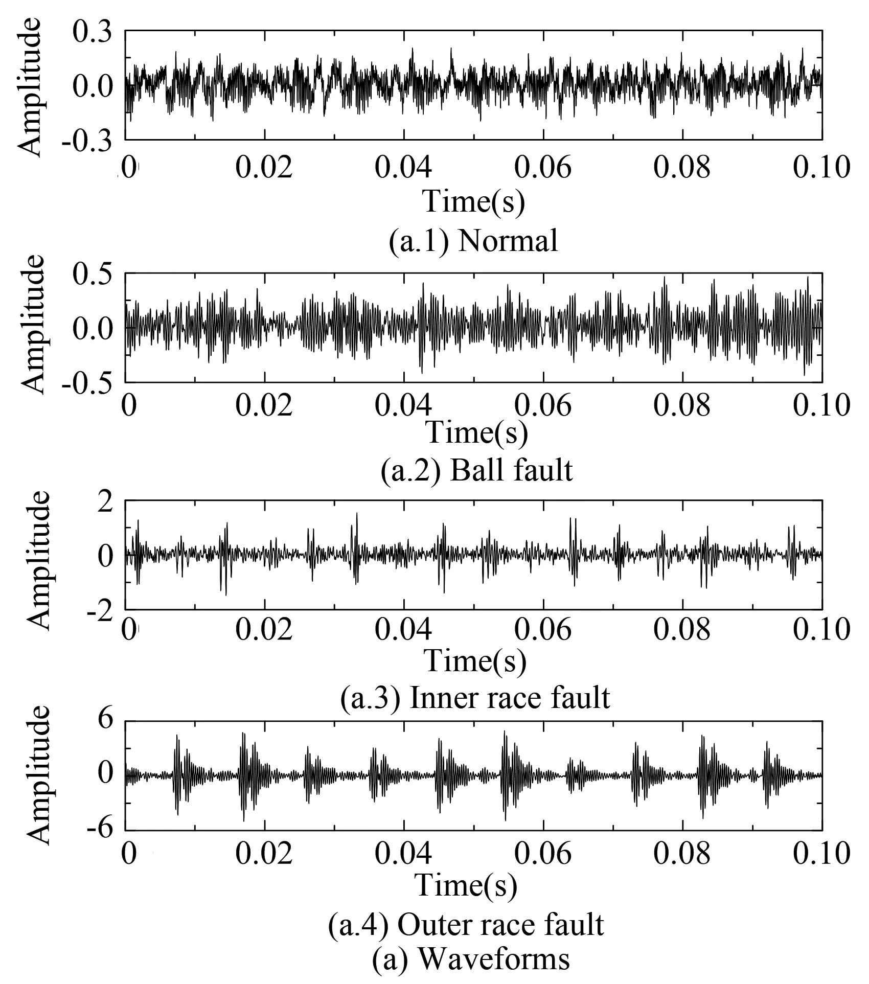
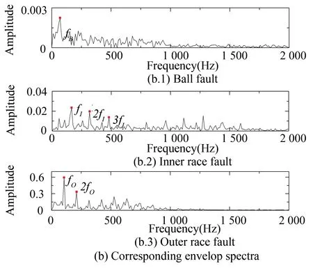
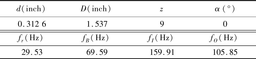
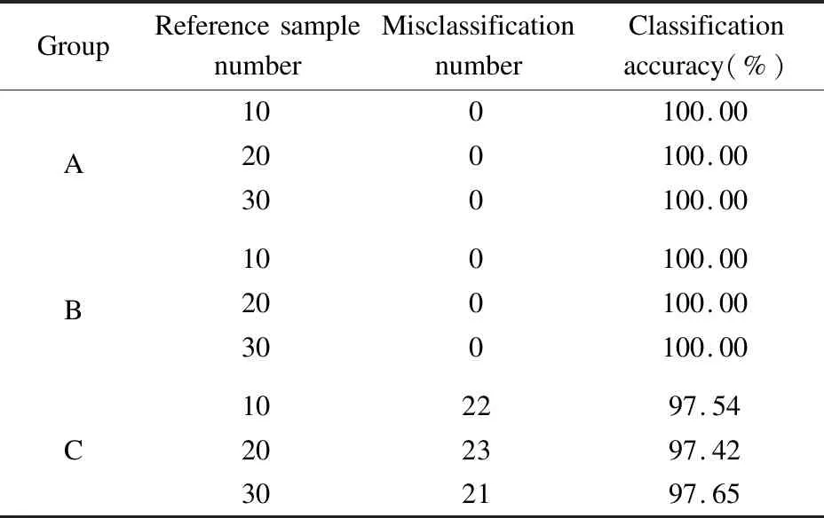
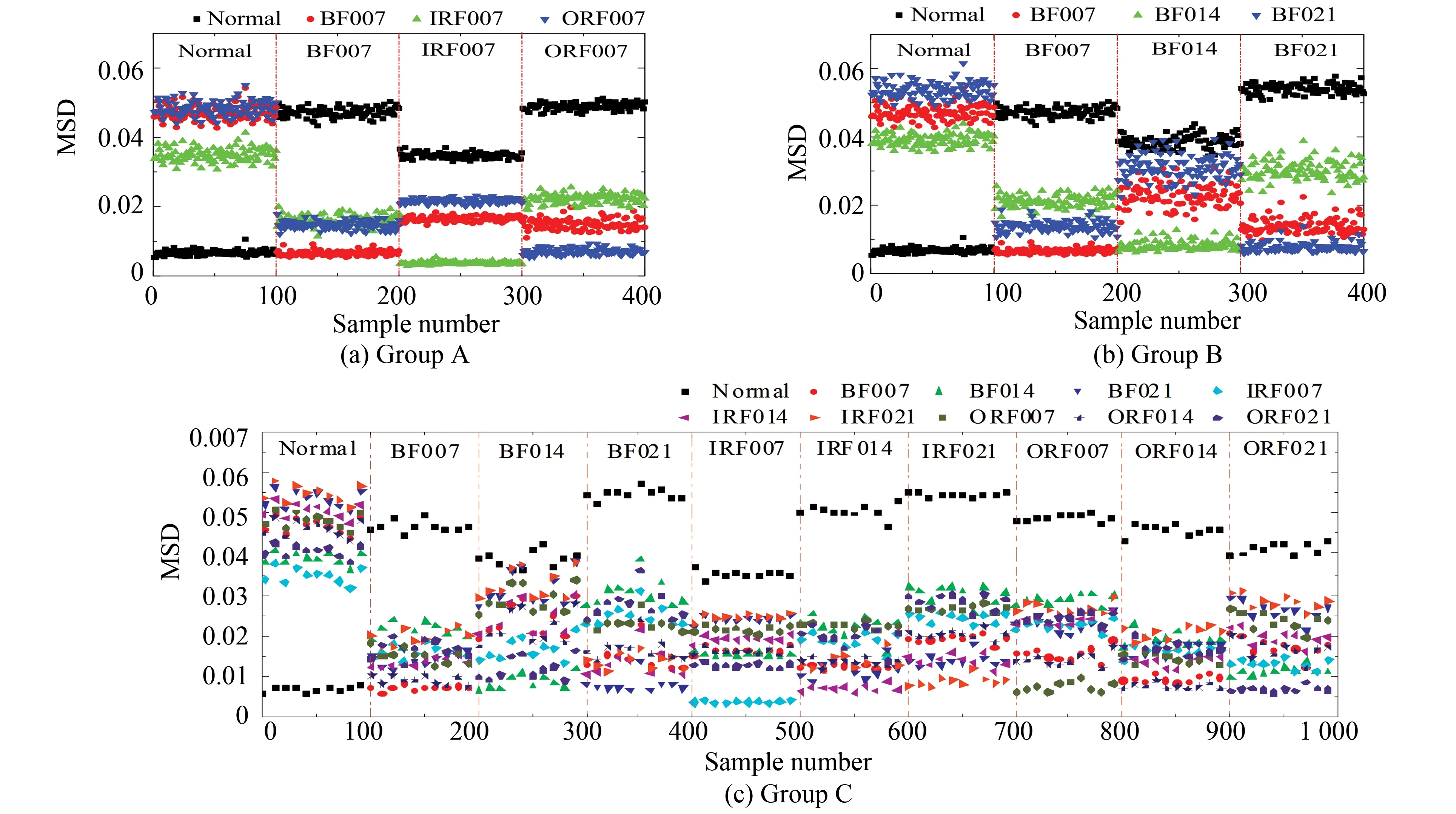
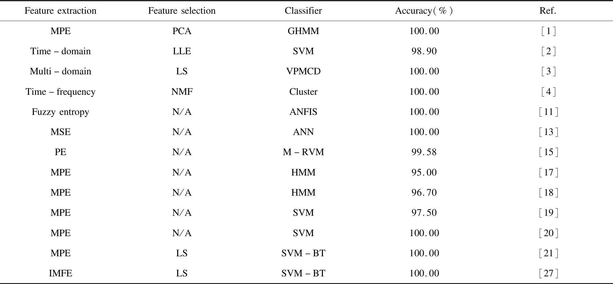
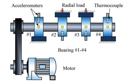
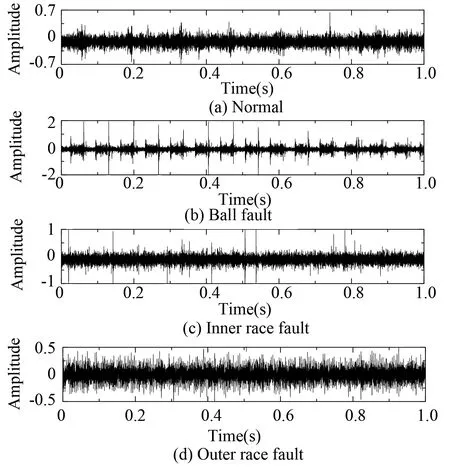
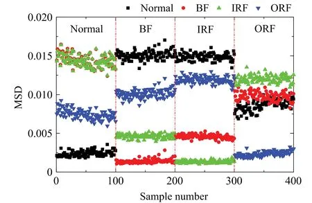
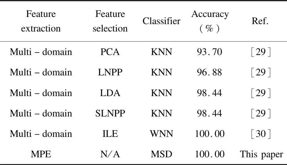
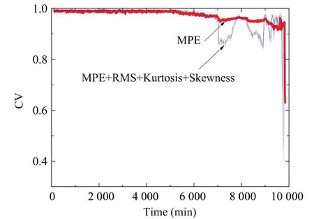
where 0≤rn≤m-1, andrn-1 x(t+rn-1τ)=x(t+rnτ) For each permutationπj,1≤j≤m!, the relative frequency can be defined as (3) (4) The MPE algorithm based on PE comprises the following two steps: (5) Fig.1 Illustration of the coarse-grained process 2) The PEs of each coarse-grained time series are calculated based on Eqs. (1)-(5) and then expressed as the function of the scale factors (6) Four parameters should be specified before using MPE, includingN,m,τ, ands. In this paper, the parameters are set asm=4,τ=1,s=20[21]. The normalized MPE is expressed as NorMPE(x,t,m,τ)=MPE(x,t,m,τ)/ (7) Considering vectors as objects, the morphology similarity distance is proposed to estimate similarity. The morphology similarity distance between twon-dimensionality vectorsLi=(li1,li2,…,lin) andLj=(lj1,lj2,…,ljn) is defined as[25] DMSD=DEuclid×(2-ASD/DManhattan) (8) whereDEuclidis the Euclid distance,DManhattanis the Manhattan distance, ASD is the absolute sum of the differences as follows: (9) The traditional index used for similarity is the Minkowski metric (10) The traditional distances Euclidean (r=2) and Manhattan distances (r=1) can be regarded as special cases of Minkowski distance. However, they both neglect the difference between vectors and fail to reflect shape similarities such as translation, compression, and stretch. For example, there are four vectors as follows: x0=(5, 5, 5),x1=(4, 4, 4) Let vectorx0be the reference vector. The vector differences, Manhattan distance, Euclidean distance, and MSD fromx1,x2, andx3tox0are computed and listed in Table 1. Table 1 Results of different distances A procedure based on MPE and MSD is established for the fault classification of rolling element bearings, and the steps are as follows: 1) Collect vibration signals of healthy and different types of fault bearings; 2) Calculate MPE values of the original signals with different fault types and construct normalized vectors as reference samples and testing samples; 3) Assign the number of the reference samples to each fault type, compute the MSD between every testing sample and all reference samples, and then average the MSD values with the specified fault; 4) Based on the nearest neighbor principle, choose the minimum value among the MSD means from all fault types, and the corresponding fault type can be identified. The flowchart of the proposed method is shown in Fig.2. Fig.2 Flowchart of the proposed method The bearing data were obtained from Bearing Data Centre of Case Western Reserve University[26]and the bearing experiment system is shown in Fig.3. During the experiment, the drive end bearing 6205-2RS JEM SKF was investigated and defective bearings were seeded with single point faults using electro-discharge machining. Vibration signals from the accelerometer were placed at the 12 o’clock position at the drive end of the motor housing with the sampling frequency 48 kHz, including normal, ball fault (BF), inner race fault (IRF), and outer race fault (ORF) (at the 6 o’clock position). Fig.3 Rolling bearing experiment system To verify the effectiveness of the proposed method, three groups of tests at defect size 0.007 inch and loading 1 HP were investigated, as depicted in Table 2, including different fault types (Group A) with waveforms shown in Fig.4(a), different defective sizes (Group B) for damage severity, and a combination of fault types and defective sizes (Group C) for complex conditions. In every condition, non-overlapping segments with lengthN=4 096 were extracted, and MPE values were computed for each segment. To illustrate specific fault types in the signal, the envelop spectra based on Teager energy operator corresponding to BF, IRF, and ORF are shown in Fig.4(b). The remarkable amplitudes occurring in the location of the fault frequencies clearly indicated the fault types. The structural parameters of the bearing are listed in Table 3, and the corresponding fault frequencies are computed as follows: Ball spin frequency (BSF) fB=0.5fr(1-d2cos2α/D2)D/d (11) Ball pass frequency on inner race (BPFI) fI=0.5fr(1+dcosα/D)z (12) Ball pass frequency on outer race (BPFO) fO=0.5fr(1-dcosα/D)z (13) wheredis the diameter of the rolling element,Dis the pitch diameter,αis the contact angle,zis the number of rolling elements, andfris the shaft speed. Table 2 Description of bearing fault groups Fig.4 Waveforms of four different conditions and corresponding envelop spectra in Group A Table3Structuralparametersofthebearingwithcorrespondingfaultfrequencies d(inch)D(inch)zα(°)0.31261.53790fr(Hz)fB(Hz)fI(Hz)fO(Hz)29.5369.59159.91105.85 Then, samples with numbers 10, 20, and 30 were utilized as reference and the rest were used for verification. The classification results are listed in Table 4. The classification accuracies reached 100%, 100%, and 97.54% in Group A, Group B, and Group C with 10 reference samples respectively, as illustrated in Fig.5. Moreover, the accuracy was not highly dependent on the number of the reference samples according to the comparison among different sample numbers in Table 4. In Fig.5(a), for example, when the bearing was normal, the mean MSD between the testing sample and the normal reference sample was the minimum, which was the same in the other three fault conditions. The four types of fault could be clearly identified based on the prominent distance between the minimum mean MSD and the other three MSDs. As illustrated in Fig.5(b), distances from the normal condition were BF014 Table 4 Classification accuracy Fig.5 Illustration of fault classification with Case 1 Table 5 A comparative study of previous work on bearing fault diagnosis published in reference Note: Improved multi-scale fuzzy entropy (IMFE); hidden Markov model (HMM); support vector machine-binary tree (SVM-BT). The data were obtained from Intelligent Maintenance System (IMS), University of Cincinnati. Four bearings were tested at one time on the same shaft in the bearing test rig as shown in Fig.6. The shaft is 2 000 r/min and a radial load of 6 000 LB is forced on the shaft with a spring mechanism. The data sampling rate is 20 kHz with the data length 20 480 points. Three groups of tests were conducted in the experiment in total and Ref. [28] can provide more details. Table 6 presents four types of fault bearings and the typical waveforms are shown in Fig.7. One hundred samples were extracted from each bearing fault condition, and 400 samples in whole were generated with lengthN=20 480. Then MPE values were computed for each sample. Fig.6 Illustration of the test rig Following the same abovementioned procedure, samples with numbers 10, 20, 30 were utilized as reference, and the rest were used for verification. The classification accuracies were all 100% with 10, 20, 30 samples, and the results are illustrated in Fig.8. A comparison of previous work considering the same four conditions as normal, BF, IRF, and ORF is listed in Table 7, which shows the advantage of the proposed method. Table 6 Description of the bearing fault group Fig.7 Waveforms of four different conditions Fig.8 Illustration of fault classification with Case 2 Table7Acomparativestudyofpreviousworkonbearingfaultdiagnosispublishedinreference FeatureextractionFeatureselectionClassifierAccuracy(%)Ref.Multi-domainPCAKNN93.70[29]Multi-domainLNPPKNN96.88[29]Multi-domainLDAKNN98.44[29]Multi-domainSLNPPKNN98.44[29]Multi-domainILEWNN100.00[30]MPEN/AMSD100.00Thispaper Note: Local and nonlocal preserving projection (LNPP); supervised-learning-based local and nonlocal preserving projection (SLNPP); linear discriminant analysis (LDA); wavelet neural network (WNN); improved Laplacian Eigenmaps (ILE); K-nearest neighbor algorithm (KNN). The whole life of Bearing 1 in Set No. 2 with ORF was employed for the investigation of damage severity. MPE values were computed at every sample time point. The first tenth points were abandoned because they were not stable at the beginning, and the confidence value (CV) was introduced as an index to evaluate the severity. A normalization function combined the Sigmoid function with MSD is introduced as[31] (14) in which the scale parameter (15) where Mean (MSDnormal) is the average of all MSDs under normal condition, and CVprecorresponds to the Mean (MSDnormal), which was determined artificially. In this paper, the scale parameterc0=10.8 and CVpre=0.99. For comparison, additional features like RMS, kurtosis, and skewness were considered, and the corresponding CV with MPE is illustrated in Fig.9. The comparison shows that the CV with MPE only was stable and could monotonously represent the damage severity along the time. Fig.9 CV with MPE only and additional features To fast and accurately diagnose the fault type in bearings, this paper presents a novel bearing fault diagnosis method based on MPE-MSD. From the above research, some conclusions are drawn as follows: 1) MPE could be employed as the representative feature for fault diagnosis and MSD is an efficient and simple approach for classification without the set-up or optimization of the tuning parameters. 2) Two experiments were performed to verify the feasibility of the proposed method. In comparison with previous studies, high accuracies were obtained in fault diagnosis for different conditions without feature selection. 3) A normalization function combining the Sigmoid function with MSD is proposed for continuous damage severity without considering full fault dataset. The degradation path shows stability and monotonicity with MPE, compared with the conditions considering MPE, RMS, kurtosis, and skewness.


2.2 Morphology Similarity Distance

x2=(5, 4, 3),x3=(5, 4, 7)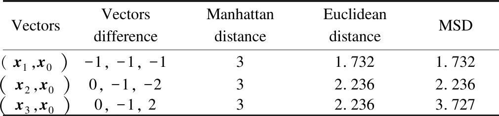
3 Procedure of Fault Diagnosis

4 Application
4.1 Case 1: Artificially Seeded Damage Bearings
4.2 Case 2: Run-to-Failure Bearings

5 Conclusions
杂志排行

Journal of Harbin Institute of Technology(New Series)的其它文章
- Role of Composite Phase Change Material on the Thermal Performance of a Latent Heat Storage System: Experimental Investigation
- GEO Satellite Thruster Configuration and Optimization
- Disturbance Observer Design with a Bode’s Ideal Filter for Sigma-Delta Modulators
- Vibration Absorption Efficiency and Higher Branches Elimination of Variable-Stiffness Nonlinear Energy Sink
- Probability Response of Shape Memory Alloy Beam Subjected to Noise Excitation
- Heat Dissipation Performance of Metal Core Printed Circuit Board with Micro Heat Exchanger