An enhanced least squares residual RAIM algorithm based on optimal decentralized factor
2020-02-24GunghuiSUNChengdongXUDnSONGYimeiJIAN
Gunghui SUN, Chengdong XU, Dn SONG, Yimei JIAN
a School of Aerospace Engineering, Beijing Institute of Technology, Beijing 100081, China
b School of Electronic and Information Engineering, Beihang University, Beijing 100191, China
KEYWORDS False alert;Least squares residual (LSR)algorithm;Missed detection;Receiver autonomous integrity monitoring (RAIM);Slope
Abstract The Least Squares Residual (LSR) algorithm is commonly used in the Receiver Autonomous Integrity Monitoring (RAIM). However, LSR algorithm presents high Missed Detection Risk (MDR) caused by a large-slope faulty satellite and high False Alert Risk (FAR) caused by a small-slope faulty satellite. In this paper, the LSR algorithm is improved to reduce the MDR for a large-slope faulty satellite and the FAR for a small-slope faulty satellite.Based on the analysis of the vertical critical slope,the optimal decentralized factor is defined and the optimal test statistic is conceived, which can minimize the FAR with the premise that the MDR does not exceed its allowable value of all three directions. To construct a new test statistic approximating to the optimal test statistic, the Optimal Decentralized Factor weighted LSR (ODF-LSR) algorithm is proposed. The new test statistic maintains the sum of pseudo-range residual squares, but the specific pseudo-range residual is weighted with a parameter related to the optimal decentralized factor.The new test statistic has the same decentralized parameter with the optimal test statistic when single faulty satellite exists,and the difference between the expectation of the new test statistic and the optimal test statistic is the minimum when no faulty satellite exists. The performance of the ODFLSR algorithm is demonstrated by simulation experiments.
1. Introduction
The integrity of Global Navigation Satellite System(GNSS)is one of the important factors to ensure the civil aviation safety.1,2There are three kinds of GNSS integrity augmentation systems: Satellite Based Augmentation System (SBAS),Ground Based Augmentation System (GBAS) and Aircraft Based Augmentation System (ABAS).3,4GBAS and SBAS can meet the integrity requirements for precision approach but would take high cost. ABAS can only meet the integrity requirements for route and non-precision approach but has been widely used for its fast response, no need for external assistance, low cost and easy implementation.
ABAS can be achieved by Receiver Autonomous Integrity Monitoring(RAIM).5The most widely used RAIM algorithm is the snapshot algorithm,6,7such as Least Squares Residual(LSR)and Parity Vector(PV)algorithms.8,9It consists of two stages: availability discrimination and satellite fault detection.Availability discrimination is achieved by comparing the Protection Level(PL)with the Alert Limit(AL)and RAIM is considered to be available with PL less than AL.10,11Satellite fault detection is performed when RAIM is available, which is achieved by consistency check using redundant measurements.12
In recent years, many researchers were devoted to improving the availability of RAIM. For example, Lee presented the Optimally Weighted Average Solution (OWAS) RAIM methods, which achieved higher availability using weights analytically derived from the position domain.13Madonna et al.developed a multi-constellation NIORAIM algorithm using non-uniform weight applied to the pseudo-range measurements involved in the position solution to reduce the protection levels.14Meng et al. improved the availability by replacing the position solution with a constellation weighted average solution.15Fan et al. proposed a new code noise and multipath distribution model to provide more accurate prior information for improving the RAIM availability.16Meng et al.proposed a new fault modes determination scheme based on feedback structure of probability accumulation to improve the RAIM availability.17
In addition,some researchers were intent on improving the fault detection probability.For example, Cho proposed a new algorithm by incorporating the relative entropy into the RAIM to improve the fault detection probability.18Li et al.proposed a new RAIM method based on robust extended Kalman filter and extrapolation-accumulation, which enhanced the fault detection probability of micro and slowly growing pseudorange bias.19Ran et al. proposed a new algorithm by combining RAIM and multivariate cumulative RAIM to increase the fault detection probability for both mutational and continuous mean shift.20Zhang et al. proposed an M-estimation RAIM method to solve the misjudgment caused by the interference from gross error to the least squares algorithm.21Yang et al.proposed an algorithm by combining the non-coherent accumulation parity vector method and the Kalman filter-based detection method.22
Both of the researches for improving the RAIM availability and the fault detection probability are effective on reducing the integrity risk. Integrity risk, also known as the Probability of Hazardous Misleading Information (PHMI), is defined as the probability that a user will experience a Position Error(PE) larger than the alert limit without an alert being raised.23,24Integrity risk is related to the prior probability of satellite fault and the probability of missed detection.25,26The probability of missed detection, also called as the Missed Detection Risk(MDR),is the key to the civil aviation safety.27The False Alert Risk (FAR) is negatively correlated with the MDR and not so important as the MDR. Therefore, these researches all ignored the FAR when they focused on reducing the MDR. However, the FAR is crucial to the continuity of GNSS.28The FAR and the MDR are decided by a geometric parameter for a satellite, which is called as the characteristic slope.29The large-slope satellite presents high MDR and low FAR while the small-slope satellite presents high FAR and low MDR.29
There were only a few researches giving consideration to both MDR and FAR. Fan proposed a slope-weighted LSR algorithm to make the test statistic keep the same trend with the position error,reducing both the MDR of large-slope satellite and the FAR of small-slope satellite, but ignored the change of the detection threshold.30Zhao et al. proposed a modified LSR algorithm based on the vertical critical slope,29but this algorithm only considered the MDR and the FAR of the vertical direction rather than those of the horizontal direction.
This paper focuses on enhancing the LSR algorithm to reduce the MDR and the FAR of the three directions in the local Cartesian (ENU) coordinate. First, the vertical critical slope is reviewed,which can define the magnitude of a vertical characteristic slope. The east and the north critical slopes are extended.Second,the optimal decentralized factor considering the critical slopes of all the three directions is defined and the optimal test statistic based on the optimal decentralized factor is derived, which can minimize the FAR with the premise that the MDR does not exceed the allowable value of all three directions.Finally,the Optimal Decentralized Factor weighted LSR(ODF-LSR)algorithm is proposed.The new test statistic of the ODF-LSR algorithm maintains the sum of pseudorange residual squares, but the specific pseudo-range residual is weighted with a parameter related to the optimal decentralized factor and the detection threshold in the ODF-LSR algorithm is reselected. The enhancement effect of the ODF-LSR algorithm on reducing the MDR and the FAR in all three directions is demonstrated by two simulation experiments compared with the LSR algorithm.
2. Critical slopes
2.1. Review of vertical critical slope
The characteristic slope for a visible satellite is defined to describe the quantity relationship between the position error and the pseudo-range residual.31The vertical characteristic slope of the ith visible satellite, labeled as VSlopei, can be calculated as23

where a3iis the ith element in the 3rd row of matrix A that is calculated by

siiis the ith diagonal element of matrix S that is calculated by

where G is the linear observation matrix in the ENU coordinate and I is a unit matrix.
The critical value of vertical characteristic slopes for all visible satellites in a geometry was proposed by Zhao et al. in 2019, which can minimize the FAR with the premise that the MDR does not exceed its allowable value of vertical.29The critical value of vertical characteristic slopes is abbreviated as the vertical critical slope in the following. Here a brief review of the derivation of the vertical critical slope is given. The derivation is based on two assumptions. The first assumption is that the pseudo-range observation noise for each visible satellite obeys the same distribution:

where P(HMI,1F)reqis the integrity risk requirement for single faulty satellite prescribed by the International Civil Aviation Organization(ICAO); K is the number of the visible satellites;Psatrepresents the prior probability of satellite fault, and Psat=10-4for GPS.33
In this paper, there are three important concepts that need to be clarified: positioning failure, missed detection and false alert3:Positioning failure is defined to occur whenever the difference between the true position and the indicated position exceeds the applicable alert limit; missed detection is defined to occur when a positioning failure is not detected; false alert is defined as the indication of a positioning failure when a positioning failure has not occurred. According to the definitions above, the theoretical calculation formula of MDR and FAR can be derived with the distribution of the Vertical Position Error (VPE) and the test statistic.
The VPE of the least squares solution obeys the distribution29:

where smmis the mth diagonal element of matrix S.
Set event A as ‘Ts <TD’ and event B as ‘VPE| |≥VAL’.TDis the detection threshold for the LSR algorithm and VAL is the vertical alert limit. According to Eq. (8) and Eq.(9), the probability of event A and event B, labeled as P(A)and P(B) respectively, can be calculated as

where f(·) represents the Probability Density Function (PDF)of Ts in Eq. (9); K-n-3 and (ξb/σ0)2smmare the freedom degrees and the decentralized parameter of non-central chisquare distribution respectively; Φ(·) represents the Cumulative Distribution Function (CDF) for the standard normal distribution.
TDis calculated by the maximum allowable probability of false alert PFA-max:

The value of a3mwill not affect the value of VSlopecriand VSlopecriis only related to the satellite-user geometry.29
2.2. East and north critical slopes
Like the vertical critical slope, there is a horizontal critical slope. Because the Horizontal Position Error (HPE) obeys two-dimensional Gauss distribution, the computation time of the horizontal critical slope is very long. Here the horizontal direction is decomposed into east and north to simplify the calculation.
By replacing the parameters in Eq.(16)with corresponding parameters in Table 1,the east critical slope and the north critical slope, labeled as ESlopecriand NSlopecrirespectively, can be calculated.
In Table 1, [RMD]aEand [RMD]aNrespectively represent the allowable value of east MDR and north MDR. EAL and NAL respectively represent the east alert limit and the north alert limit.
[RMD]aEand [RMD]aNcan be calculated as

Table 1 Parameter correspondence.

where[RMD]aHrepresents the allowable value of the horizontal MDR, which is calculated by

The value of EAL and NAL can be calculated according to the value of HAL.For example,LPV-200,which means Localizer Performance with Vertical guidance down to 200 feet,stipulates that the Horizontal Alert Limit (HAL) equals 40 m but does not stipulate the EAL and the NAL.The area defined by the HAL is a circle,of which the radius is 40 m and the center is at the origin in the horizontal position error coordinate.The edge length of the largest square inside the circle is slightly larger than 56 m. Under the premise that the east MDR and the north MDR do not exceed [RMD]aEand [RMD]aNrespectively,the value of the EAL and the NAL are both set as 28 m to ensure that the horizontal MDR decided by HAL does not exceed [RMD]aH. Here a brief proof is given. For convenience of explanation, a series of events are set in Table 2.
In Table 2,HPE,EPE and NPE respectively represent horizontal position error, east position error and north position error.
According to Table 2, two kinds of the horizontal MDR can be calculated. One is decided by HAL stipulated in LPV-200 and the other is decided by EAL and NAL, which are both set as 28 m.
The horizontal MDR decided by HAL, labeled as RMDH,can be calculated as

The two-dimensional joint PDF of HPE is labeled as fN(x,y), and then
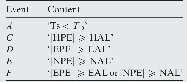
Table 2 Event setting.

Now the magnitude of the characteristic slope in each direction can be defined. The characteristic slope larger than the critical slope in the corresponding direction can be defined as a large slope whereas the characteristic slope smaller than the critical slope of the corresponding direction can be defined as a small slope. Further,the faulty satellite with a large slope in any direction can be defined as a large-slope faulty satellite and the faulty satellite with small slopes in all directions can be defined as a small-slope faulty satellite.
3. Optimal test statistic
3.1. Derivation of optimal test statistic
VSlopecrican minimize the FAR with the premise that the MDR does not exceed its allowable value of vertical. According to Eq.(1)and Eq.(10),the decentralized parameter corresponding to VSlopecri, labeled as λVcri, can be obtained:

Then the optimal test statistic considering the MDR and the FAR in the three directions, labeled as Tsopt, can be defined. When no faulty satellite exists, Tsoptshould obey astandard chi-square distribution, and when there is a single faulty satellite VSF, Tsoptshould obey non-central chi-square distribution with the decentralized parameter of λopt.
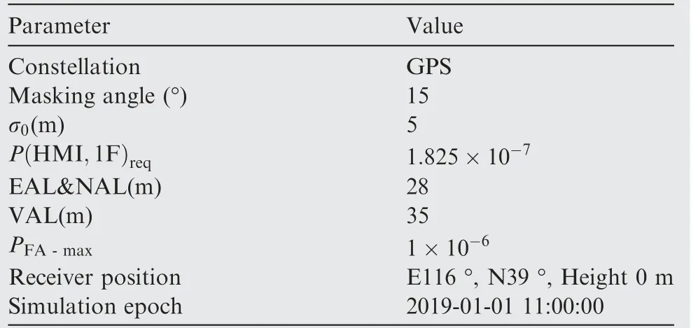
Table 3 Simulation scenario.
3.2. Performance verification of optimal test statistic
A simulation experiment is carried out to verify the performance of Tsopt. The simulation scenario is shown in Table 3.There are 10 visible satellites in this scenario. PRN 2 and PRN 13 are respectively set as the single faulty satellite as the representative of large-slope and small-slope satellites.
As seen in Table 4, ESlopem>ESlopecriand VSlopem>VSlopecrifor PRN2,and thus PRN2 meets the condition of a large-slope satellite; ESlopem<ESlopecri,NSlopem<NSlopecriand VSlopem<VSlopecrifor PRN13,and thus PRN13 meets the condition of a small-slope satellite.For LPV-200,the overall integrity requirement is that P(HMI)must not exceed 2×10⁻⁷per approach, that is P(HMI)req=2×10⁻⁷, which includes the contribution for the horizontal and vertical dimensions.35P(HMI,1F)reqis obtained by subtracting the integrity risk requirement for no faulty satellites and multiple faulty satellites from the overall integrity requirement.32
The comparison of lgRMDand lgRFAcurves for these two faulty satellites in the three directions using Ts and Tsoptare shown in Fig. 1 and Fig. 2. In the two figures, the horizontal axes represent the observation bias and the vertical axes represent the logarithms of MDR and FAR in the three directions respectively.
As seen in Fig.1,only the lgRMDNcurve of Ts is lower than the lg[RMD]aNcurve whereas the lgRMDEand the lgRMDVcurves of Ts intersect with the lg[RMD]aEand the lg[RMD]aVcurves respectively.The lgRMDcurves of Tsoptare all lower than those of Ts. Particularly, the lgRMDVcurve of Tsoptis tangent to the lg[RMD]aVcurve,which means that the maximum value of vertical MDR does not exceed its allowable value exactly.And the lgRMDEand the lgRMDNcurves of Tsoptare lower than the lg RMD[ ]aEcurve and the lg RMD[ ]aNcurve respectively. On the other hand,the lgRFAcurves of Tsoptare all higher than those of Ts. Fig. 1 shows that Tsoptcan reduce the MDR for largeslope faulty satellites to below the allowable value at the cost of increasing the FAR in the three directions.
As seen in Fig.2,the lgRMDcurves of Ts are all lower than the lg RMD[ ]acurves. The lgRMDcurves of Tsoptare all higher than those of Ts.Particularly,the lgRMDEcurve of Tsoptis tangent to the lg RMD[ ]aEcurve, which means that the maximum value of east MDR does not exceed its allowable value exactly.And the lgRMDNand the lgRMDVcurves of Tsoptare lower than the lg RMD[ ]aNand the lg RMD[ ]aVcurves respectively. On the other hand, the lgRFAcurves of Tsoptare all lower than those of Ts.Fig.2 shows that Tsoptcan minimize the FAR for smallslope faulty satellites with the premise that the MDR does not exceed the allowable values in the three directions.

Table 4 Parameters of PRN2 and PRN13.
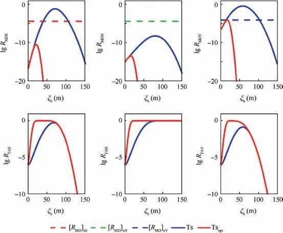
Fig. 1 RMD and RFA of PRN2 for Ts and Tsopt.

Fig. 2 RMD and RFA of PRN13 for Ts and Tsopt.
4. ODF-LSR algorithm
Tsoptis unable to be constructed because among all test statistics constructed by the pseudo-range residual, only Ts obeys a standard chi-square distribution with no faulty satellite while the decentralized parameter of Ts with single faulty satellite is not equal to λopt. However, a new test statistic approximating to Tsopt, can be constructed. The decentralized parameter of the new test statistic is equal to λoptwhen single faulty satellite exists. Besides, the difference between the expectation of the new test statistic and Tsoptis the minimum when no faulty satellite exists.The LSR algorithm is enhanced on reducing the MDR of large-slope faulty satellites and the FAR of smallslope faulty satellites using the new test statistic. Because the new test statistic is constructed by weighting the specific pseudo-range residual with a parameter related to cdopt, the enhanced LSR algorithm is abbreviated as ODF-LSR algorithm, where ODF represents ‘‘optimal decentralized factor”.
4.1. The most potentially faulty satellite
According to Eqs.(40)-(42),λoptis related to a1m,a2mand a3m,the parameters of the faulty satellite VSF.However, the faulty satellite is initially unknown. Here the correlation analysis method, which was proposed to evaluate the correlation between the observation error and the residual vector, is used to judge the most potentially faulty satellite(labeled as VSM).36The details of judging the most potentially faulty satellite, are described in Appendix A. The following derivation assumes that the mth visible satellite is the only faulty satellite in all visible satellites and its observation bias is ξb. In the practical fault detection,the serial number of the most potentially faulty satellite VSMwill be taken as the prior estimate of m.
4.2. Test statistic for ODF-LSR algorithm
The weighted coefficient, which can make the decentralized parameter of the new test statistic equal to λoptwhen single faulty satellite exists, is introduced in this section.
The test statistic of ODF-LSR algorithm, labeled as Tsd,is constructed as

Referring to the decentralized parameter of Ts for the LSR algorithm,that of Tsdcan be defined as the difference between E[Tsd]with one and no faulty satellite,labeled as λd.Subtracting Eq. (47) from Eq. (48), we have

4.3. Selection of β position
Analyzing Eq.(44),the specific value of l actually refers to the position of β in the weighted matrix P.To minimize the difference between the expectation of Tsdand Tsoptwhen no faulty satellite exists, the value of l is decided as follows.
According to Eq. (47), the difference between the expectations of Tsdand Ts with no faulty satellite is

4.4. Detection threshold and process for ODF-LSR algorithm
Considering that Tsddoes not obey a standard chi-square distribution when no faulty satellite exists, the test threshold of ODF-LSR algorithm, labeled as TDd, should be reselected rather than using TDof LSR algorithm directly.
Theoretically,TDdshould be reselected according to the following equation:

The detection process of ODF-LSR algorithm is presented in Fig. 3.
As seen in Fig. 3, the process of the ODF-LSR algorithm can be divided into 4 steps in general.
Step 1. Calculate the pseudo-range residual vector ω,matrix A, matrix S and the critical slopes in the three directions.
Step 2. Search the most potentially faulty satellite VSM.
Step 3.Calculate the weighted matrix P,including the optimal decentralized factor cdopt, the weighted position l and the weighted coefficient β.
Step 4. Calculate the test statistic Tsdand the detection threshold TDdfor fault detection.
It should be noted that the numerical calculation of Slopescriwill takes a certain time (usually tens of seconds). It is difficult to update Slopescriin real time. Fortunately,Slopescrihave one-to-one correspondence with ai(i=E,N,V)at the fixed AL, TD, σ0and K-n. Hence Slopescrican be off-line calculated for all possible aivalues and saved in the receiver. And the receiver can match Slopescriaccording to on-line calculation result of ai.32
5. Results
One detection example and one simulation experiment are carried out to respectively display and demonstrate the performance of the ODF-LSR algorithm compared with the LSR algorithm.
5.1. Detection example
The performance of the ODF-LSR algorithm is analyzed through two detection examples, which use real data collected by receiver.The scenario of the detection examples is shown in Table 5. The large-slope satellite PRN24 is set as the faulty satellite in the first example and its pseudo-range is injected 40 m bias. The small-slope satellite PRN13 is set as the faulty satellite in the second example and its pseudo-range is injected 5 m bias. The detection results are presented in Fig. 4 and Fig. 5, and two sub figures present the position errors in the three directions and the ratio of the test statistic to its threshold, labeled as Ts/Td.

Fig. 3 Detection process for ODF-LSR algorithm.
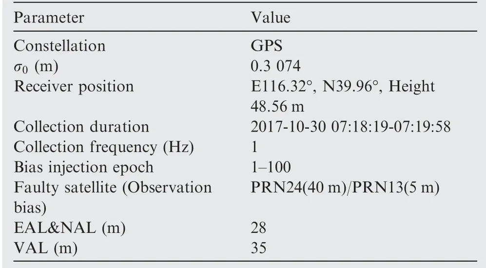
Table 5 Simulation scenario.

Fig. 4 PE and Ts/Td for PRN24 as faulty satellite.

Fig. 5 PE and Ts/Td for PRN13 as faulty satellite.
The geometry does not vary significantly during the detection. ESlopecri, NSlopecri, VSlopecri, a1m, a2mand a3mcan be considered as a constant and cdoptcan be calculated according to the geometry at the start epoch of detection. In the result analysis, missed detection is defined as the state that any position error exceeds the alert limit while Ts/Td <1;false alert is defined as the state that all the position errors do not exceed the alert limit while Ts/Td >1.
In Fig. 4, the pseudo-range injected bias of PRN24 makes the position errors change significantly. The NPE exceeds NAL and a positioning failure occurs.According to the definition of the missed detection in Section 2.1,the value of Ts/Td should exceed 1, otherwise the missed detection will occur. As seen in Fig.4,the value of Ts/Td for the ODF-LSR algorithm mostly exceeds 1 and is greater than that for the LSR algorithm overall. The statistical results show that among the 100 epochs, the frequency of missed detection and false alert for the ODF-LSR algorithm are 35 and 0 respectively, whereas those for LSR algorithm are 49 and 0. Compared with the LSR algorithm, the MDR for large-slope faulty satellites is reduced using the ODF-LSR algorithm.
In Fig.5,the pseudo-range injected bias of PRN13 brings a little change in the position errors. All the position errors do not exceed the corresponding alert limits and no positioning failure occurs. According to the definition of the false alert in Section 2.1, the value of Ts/Td should not exceed 1, otherwise the false alert will occur. As seen in Fig. 5, the value of Ts/Td for the ODF-LSR algorithm does not exceed 1 while the value of Ts/Td for the LSR algorithm mostly exceeds 1.The statistical results show that among the 100 epochs, both the frequency of missed detection and false alert for the ODF-LSR algorithm are 0, whereas those for the LSR algorithm are 0 and 57. Compared with the LSR algorithm, the FAR for small-slope faulty satellite is reduced using the ODF-LSR algorithm.
Fig. 4 and Fig. 5 show the performance of the ODF-LSR algorithm intuitively. Compared with the LSR algorithm, the ODF-LSR algorithm can reduce the MDR for large-slope faulty satellites and reduce the FAR for small-slope faulty satellites.
5.2. Contrast simulation
The optimization effect of the ODF-LSR algorithm is demonstrated by the contrast simulation, which is carried out in the scenario shown in Table 3. The observation noise is set as 0 mean white Gaussian noise with a standard deviation of 5 m.To obtain the MDR and the FAR of ODF-LSR and LSR algorithms, 1×10⁶times of simulations are completed for RRN2 and PRN13 respectively with observation bias from 1σ0to 20σ0. According to Eq. (14) and Eq. (15), the MDR and the FAR are determined by P(A)and P(B).In this experiment, P(B) is calculated by Eq. (12), while P(A) is calculated by statistics. Simulation results are presented in Figs. 6-9, in which the horizontal axes represent the observation bias,times of σ0and the vertical axes represent the MDR and the FAR in the three directions respectively.
In Fig. 6, the lgRMDcurves of Tsdare all lower than those of Ts,but the lgRMDNand the lgRMDVcurves still intersect with the lg RMD[ ]aNand the lg RMD[ ]aVcurves respectively. In Fig. 7,the lgRFAcurves of Tsdare all higher than those of Ts. The results show that the ODF-LSR algorithm can reduce the MDR for a large-slope faulty satellite at the cost of increasing the FAR in the three directions but cannot reduce them to below the allowable values.
The curves in Fig.8 are incomplete because the MDR at the corresponding points is close to zero and logarithm of zero cannot be calculated. In Fig. 8, the lgRMDcurves of Tsdare all higher than those of Ts. In addition, the lgRMDVcurve is approximately tangent to the lg RMD[ ]aVcurve. In Fig. 9, the lgRFAcurves of Tsdare all lower than those of Ts. The results show that the ODF-LSR algorithm can reduce the FAR for a small-slope faulty satellite with the premise that the MDR does not exceed the allowable value in the three directions.

Fig. 6 RMD for PRN2 using different algorithms.

Fig. 7 RFA for PRN2 using different algorithms.

Fig. 8 RMD for PRN13 using different algorithms.

Fig. 9 RFA for PRN13 using different algorithms.
Depending on the above analysis,the ODF-LSR algorithm has a significant optimization effect on reducing MDR and FAR compared with the LSR algorithm. Moreover, the optimization considers all three directions. However, Tsdfails to achieve the detection performance of Tsoptas expected. The optimization effect of the ODF-LSR algorithm for smallslope faulty satellites is ideal, while that for large-slope faulty satellites needs to be improved.
6. Conclusions
In this paper, the ODF-LSR algorithm is proposed to reduce the MDR caused by the large-slope faulty satellite and the FAR caused by the small-slope faulty satellite considering all three directions.
(1) The east and the north critical slopes are expanded according to the vertical critical slope, which is the largest one making the vertical MDR not exceed its allowable value.
(2) The optimal decentralized factor unifying the properties of the three critical slopes is defined and the optimal test statistic based on the optimal decentralized factor is conceived, which can minimize the FAR with the premise that the MDR does not exceed the allowable value of all three directions.
(3) The Optimal Decentralized Factor weighted LSR(ODF-LSR) algorithm is proposed to construct a test statistic approximating to the optimal test statistic. It has been proved in theory that when single faulty satellite exists, the new test statistic has the same decentralized parameter with the optimal test statistic, and when no faulty satellite exists, the difference between the expectation of the new test statistic and the optimal statistic is the minimum.
(4) The performance of the ODF-LSR algorithm is demonstrated by a detection example and a simulation experiment. The ODF-LSR algorithm can reduce both the MDR caused by the large-slope faulty satellite and the FAR caused by the small-slope faulty satellite in the three directions. Particularly, the FAR caused by the small-slope faulty satellite can be minimized with the premise that the MDR does not exceed the allowable values.
Appendix A

Appendix B
Under the assumption of no faulty satellite, ωlin Eq.(45) can be expressed as


杂志排行
CHINESE JOURNAL OF AERONAUTICS的其它文章
- Design and experimental study of a new flapping wing rotor micro aerial vehicle
- CFD/CSD-based flutter prediction method for experimental models in a transonic wind tunnel with porous wall
- Prediction of pilot workload in helicopter landing after one engine failure
- Study of riblet drag reduction for an infinite span wing with different sweep angles
- Modulation of driving signals in flow control over an airfoil with synthetic jet
- Strong interactions of incident shock wave with boundary layer along compression corner
