Prediction of pilot workload in helicopter landing after one engine failure

Zhiming YU, Xufei YAN,b, Renling CHEN,*

a National Key Laboratory of Rotorcraft Aeromechanics,Nanjing University of Aeronautics and Astronautics,Nanjing 210016,China

b Intelligent Robot Research Center, Zhejiang Lab, Hangzhou 310000, China

KEYWORDS Engine failure;Nonlinear optimal control method;Pilot control activity;Pilot workload;Wavelet transform analysis

Abstract This paper presents a method to predict the pilot workload in helicopter landing after one engine failure. The landing procedure is simulated numerically via applying nonlinear optimal control method in the form of performance index,path constraints and boundary conditions based on an augmented six-degree-of-freedom rigid-body flight dynamics model, solved by collocation and numerical optimization method.UH-60A helicopter is taken as the sample for the demonstration of landing after one engine failure.The numerical simulation was conducted to find the trajectory of helicopter and the controls from pilot for landing after one engine failure with different performance index considering the factor of pilot workload. The reasonable performance index and corresponding landing trajectory and controls are obtained by making a comparison with those from the flight test data.Furthermore,the pilot workload is evaluated based on wavelet transform analysis of the pilot control activities. The workloads of pilot control activities for collective control, longitudinal and lateral cyclic controls and pedal control during the helicopter landing after one engine failure are examined and compared with those of flight test.The results show that when the performance index considers the factor of pilot workload properly,the characteristics of amplitudes and constituent frequencies of pilot control inputs in the optimal solution are consistent with those of the pilot control inputs in the flight test.Therefore,the proposed method provides a tool of predicting the pilot workload in helicopter landing after one engine failure.

1. Introduction

A considerable portion (approximately 50%) of helicopter accidents are caused by engine failure. According to statistics,1,2there is one engine failure in every 10,000 hours of operation. Therefore, the safety is one of the critical issues for helicopter encountering One Engine Inoperative (OEI) situation.In general,flight tests are the ultimate methods to obtain the safe landing procedures. However, they are very risky,time-consuming and expensive to conduct. In order to reduce the risks and costs,optimal control method has been proposed to predict the optimal safe landing procedure in OEI to provide a benchmark of optimal maneuvers for flight tests. A number of works have studied the helicopter optimal landing procedures in OEI situations using optimal control method to explore the mechanism of OEI problem. Johnson3, Lee4and Chen and Zhao5used two-dimensional point-mass models to investigate the optimal trajectories for twin engine helicopters in one engine inoperative situations. Aponso used trajectory optimization method to show the capability of providing helicopter pilots with guidance and training.6,7Okuno et al.applied nonlinear optimal control theory to a longitudinal rigid-body model to predict the unsafe region(height-velocity diagram) and to study the optimal landing procedures for the given initial flight conditions.8Bottasso,9Bibik10and Meng11et al. studied the optimal control of helicopter in one engine failure based on six-degree-of-freedom rigid-body models to provide more valuable information on flight trajectory and control strategy. Based on the aforementioned studies, it seems worthwhile to study the OEI problem more deeply by means of the analysis of pilot workload in helicopter landing optimization after one engine failure. Helicopter landing in OEI is a multi-axis maneuver with highly complex pilot control process. The high pilot workload may threaten the safe flight throughout the landing procedure.This paper intends to find a method that can be used to evaluate the pilot workload of helicopter landing optimization in OEI.

The helicopter landing optimization after one engine failure is studied by applying nonlinear optimal control method. An augmented six-degree-of-freedom rigid-body flight dynamics model is built and validated against the flight test data and the AMES GEN HEL model.12UH-60A helicopter landing procedure in OEI is taken as the example. Considering safety-related requirements and helicopter performance limits,the optimal landing procedure is formulated as a Nonlinear Optimal Control Problem(NOCP)in the form of performance index, path constraints and boundary conditions, solved by collocation and numerical optimization method. The optimal landing procedure is compared with the flight test data in Ref. 13. Finally, the pilot control activities are quantified and evaluated by applying wavelet analysis method based on the pilot control inputs of the optimal solution and the flight test data.14,15The pilot workloads are also compared and discussed.

2. Augmented flight dynamics model

2.1. Modeling

An augmented six-degree-of-freedom rigid-body flight dynamics model is used for landing optimization after one engine failure. The aerodynamic loads on the fuselage, vertical tail and horizontal stabilizer are obtained based on wind tunnel test data. The aerodynamic forces and moments acting on the main rotor are calculated using the blade element method with ground effect. The aerodynamic interference between rotor and airframe is included based on wind tunnel test data. The detailed formulation of the mathematical model can be obtained in Refs. 11,16. A brief description is provided here.

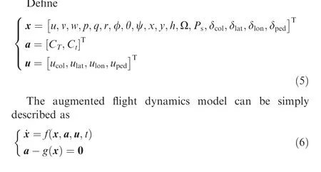
The basic flight dynamics model is given with six degrees of freedom: three translational motions and three angular motions. The state variables are velocity components of body axes(u,v,w),attitude angle rates(p,q,r),attitude angles(φ,θ,ψ) and positions (x, y, h). The control variables are pilot controls(range 0-1)of collective stick input δcol,lateral and longitudinal stick inputs (δlat,δlon) as well as pedal input δped. The governing equations are derived and summarized below:

where Pmr, Ptrare the required power of main rotor and tail rotor respectively, η is the helicopter power efficient factor,IMR, ITRare the polar moments of inertia of main rotor and tail rotor respectively,k is the ratio of nominal tail rotor angular speed to nominal main rotor angular speed, tpis the turboshaft engine time constant, and POEIis the one engine inoperative power available.

For computational efficiency in the numerical optimization,the aerodynamic thrusts of main and tail rotors Tmrand Ttrare used as algebraic variables, and the corresponding algebraic equations are

where ρ is the air density, R and Rtare the main rotor radius and tail rotor radius respectively,CTand Ctare the main and tail rotor thrust coefficients respectively, κ is the tip-loss factor of main rotor blades, a is the main rotor blade lift-curve slope, σ is the main rotor solidity ratio,θ0is the main rotor collective pitch, (μx, μy, μz) are the dimensionless velocity components of main rotor hub in the shaft axes, θ1is the main rotor blade twist angle, λ is the main rotor inflow ratio,θcis the lateral cyclic pitch, θsis the longitudinal cyclic pitch,(ωx, ωy, ωz) is the dimensionless angular velocity components of helicopter in the shaft axes, atis the tail rotor blade liftcurve slope, σtis the tail rotor solidity ratio, θtis the tail rotor collective pitch, θ1tis the tail rotor blade twist angle,μtis the tail rotor advance ratio, and λtis the tail rotor inflow ratio.

In order to account for the limits on control rates and to avoid jump discontinuities arising in the time history of controls in the numerical optimization,9,11time derivatives of δcol, δlat, δlonand δpedare applied as the control variables,denoted byucol, ulat, ulonand uped. In the meantime, δcol, δlat,δlonand δpedare regarded as the portion of the state variables.The corresponding differential equations can be expressed as

Helicopter landing procedure after one engine failure is a kind of maneuvering flight process with urgency. In order to improve maneuverability, the Stability and Command Augmentation System (SCAS) is usually turned off in the current researches on helicopter OEI problem.9-11,13Therefore the model in this paper does not consider the SCAS.

Eqs. (1)-(4) are the governing equations of the augmented six-degree-of-freedom rigid-body flight dynamics model for landing optimization in OEI, which can be described as a set of Differential-Algebraic Equations (DAE) with differential Eqs. (1), (2), (4) and algebraic Eq. (3).

2.2. Validation

The data of flight test and AMES GEN HEL model of UH-60A helicopter in Ref. 12 are utilized to validate the augmented flight dynamics model in steady-state flight conditions at altitude of 1600 m and gross weight of 7257 kg.Fig.1 shows the comparison between the predicted results and the flight test data as well as the AMES GEN HEL model. It can be seen that the steady-state variables calculated are in good agreement with the flight test data and the AMES GEN HEL model.

In order to verify the accuracy of the proposed model in dynamic response, the transient responses of the AMES GEN HEL simulation in Ref. 12 for one inch right cyclic control input at hover were taken for comparison. The control inputs shown in Fig. 2(a) as well as the flight conditions such as weight, center of gravity, inertial moments and atmospheric environment are all the same as those of Ref. 12 for the calculation of transient responses. Fig. 2(b) shows the comparison of the calculated transient responses of translational velocities, angular velocities and attitudes with those of the AMES Gen Hel simulation. It can be found that the proposed model can capture the UH-60 helicopter dynamic characteristic and has the enough accuracy in the dynamic responses.

3. Formulation of nonlinear optimal control problem

This paper focuses on the case of helicopter landing trajectory and control process optimization in one engine failure situation. The helicopter is assumed in a steady state under standard atmospheric conditions before OEI. After a short time of pilot response delay,the subsequent safe landing procedure can be described as to arrive at the ground within the permitted state limits subject to a safe, feasible flight path. To the end, the landing procedure can be formulated as a Nonlinear Optimal Control Problem (NOCP), which can be expressed as follows.

3.1. Optimal variables

Optimal variables include differential state variables x, algebraic states a, control variables u of the augmented flight dynamics model and the free final time tf.

3.2. Cost function

The cost function of NOCP is the performance index of whole landing procedure in OEI, which can be formulated into the following expression. Function φ represents the performance index item of states at boundary (initial and terminal), and function L represents the performance index item of states and controls in the whole control process.

The determination of specific performance index J needs to interpret the effects of multiple factors, such as the time of flight,safety,feasibility and pilot workload.Therefore,the performance index is usually expressed as a weighted and normalized combination of various factors. The corresponding weighting coefficient is specified according to the degree of importance of each item. For the performance index function φ at boundary, we need to consider the weighting of each target term at the end of the landing procedure, and for the performance index function L in the optimal control process, we need to consider the weighting of each target term in the whole landing procedure.

This paper will determine each target item according to the specific flight task from Ref. 13 in the case study. The simulation results are used to analyze the effects of various weight coefficients on the landing procedure, pilot control activity and pilot workload.

Fig. 1 Model trim validation with flight data and AMES GEN HEL model.

The NOCP can be successfully solved if the time history of the control vector u（t ） that minimizes the cost function is found under the following constraints.

3.3. Constraints

The constraint equations consist of differential equations, initial boundary conditions, path constraints and terminal constraints.

Differential equations are the differential part of the DAE system (6),

The initial boundary conditions att0are determined in the moment of initial pilot control actuation after OEI. Normally, pilot response delay time tdshould be considered and applied for NOCP after OEI before pilot operation.17During the delay period, the pilot is assumed to hold the controls fixed. In order to obtain the initial boundary conditions (xdelay, adelay, udelay) at time t0, the differential equations are integrated for tdat the moment of OEI with controls fixed to the initial trim values, using backward differentiation formulae. The initial boundary conditions at t0can be described as

The path constraints of states are properly selected according to the safety-related requirements and helicopter performance limits, and the constraints of the pilot control rates are chosen according to the constraints in Ref. 9 for Category-A helicopter safe flight after one engine failure,

In addition, the algebraic part of the DAE system (6) is used as path equality constraints,

The terminal constraints at tfare properly selected according to the specific requirements of FAR for rotorcraft landing situations,17

4. Numerical solution techniques

The state and control variables of the NOCP for helicopter landing in OEI are numerous, and the cost function as well as the constraints are very complicated.Therefore,the optimal solution needs to be solved numerically.To improve computational efficiency and rate of convergence in the numerical optimization, the optimal variables of the NOCP are normalized and scaled first as follows:

where Ω0is the nominal rotor rotation speed.

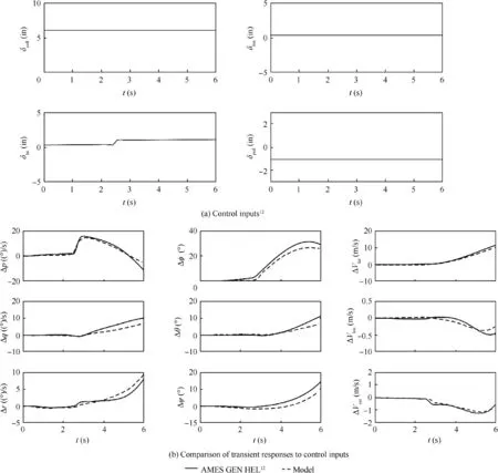
Fig. 2 Model dynamic response validation with AMES GEN HEL model.

In order to make the normalized-scaled optimal variables close to one in value,take kx=10 and kv=0.1.The governing equations of the normalized and scaled augmented flight dynamics model can be expressed as

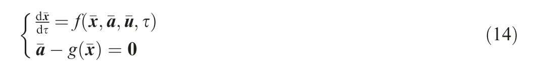
where

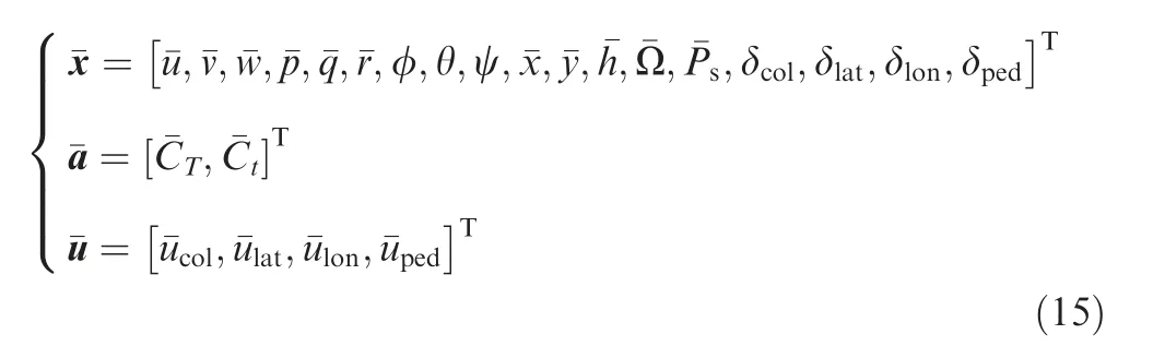
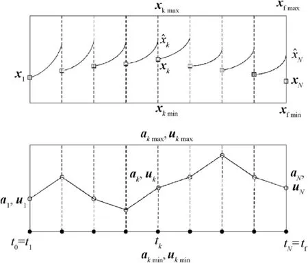
Fig. 3 Direct multiple shooting approach.

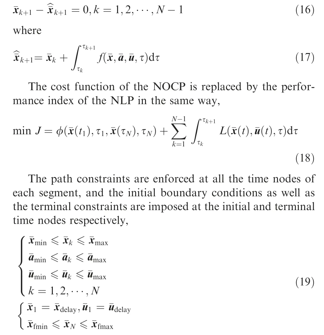
At present,the most effective and flexible approach to solve NOCP is to convert it into a Nonlinear Programming (NLP)problem via a collocation approach,which can be then solved with nonlinear programming algorithm.In this paper,a collection approach called direct multiple shooting is used to transcribe the NOCP directly into a discrete NLP by breaking the states and controls of the continuous procedure into shorter time segments.18,19This approach is typically used in the applications of high complexity and/or a large number of degrees of freedom.19

The fundamental idea of direct multiple shooting approach is shown in Fig. 3, the solution time interval [τ0, τf] of the NOCP is divided into N-1 equal time segments. For time segment k, we can integrate the differential equations from τkto the end of the segment at τk+1using time stepping approach with piecewise linear interpolation ofandwhich helps to decrease the computational cost of finite differencing by increasing the problem sparsity. The multiple shooting segments are used for stabilizing the integration of vehicle motion equations. This is particularly important when analyzing unstable systems, which is often the case when considering rotorcraft vehicles.

Denote the result of this integration byand thus the shooting of segment k can be represented by

The optimal solution of NOCP can be obtained by solving the NLP using Sequential Quadratic Programming (SQP)method described in Ref. 20. Finally, piecewise linear interpolation is used to construct an approximation to the continuous optimal control process u（t ）of the NOCP,and the approximation of the continuous optimal states x（t ）are obtained by integrating the differential equations from t0to tf.

5. Helicopter landing optimization after one engine failure

In this paper, UH-60A helicopter landing procedure in OEI is taken as the example. The initial OEI conditions from the flight test in Ref. 13 are set to conduct the calculation for the result comparison. The conditions are steady-state with weight of 7239 kg, altitude of 9.1 m, standard atmospheric environment, forward speed of 0 m/s, track angle of 0°, no sideslip and pilot delay time of 1.2 s. The landing procedure lasted about 5 s because the altitude was set low for safe landing during OEI.

Considering the safety, feasibility of landing procedure in OEI and the limitation of pilot control rates, the specific path constraints and terminal constraints are chosen according to the corresponding constraints in Ref. 9 for Category-A helicopter safe flight after one engine failure.

The specific path constraints are as follows:

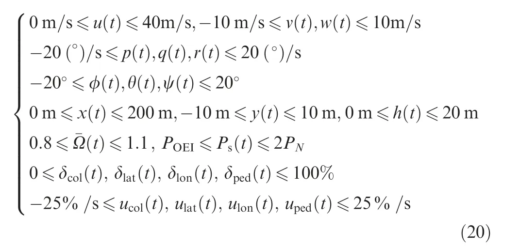
where PNis the rated power of one engine.

The terminal constraints are

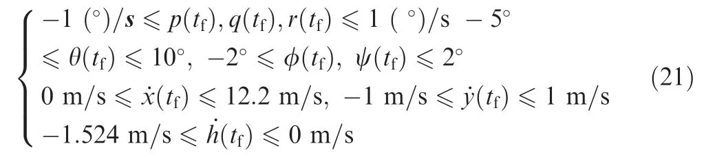
In the determination of performance index, firstly, as an emergency maneuver, it would be better if pilot can land the helicopter as soon as possible within the safe range so that the flight time should be included in the performance index.In addition,since the object of the study is a piloted helicopter,pilot workload should also be considered to avoid too aggressive manipulations. Therefore, the performance index in this study can be written as

where τ0,τfare the normalized-scaled initial and terminal time respectively, wtis the time weight coefficient, wpis the pilot workload weight coefficient, and wcol, wlat, wlonand wpedare the corresponding weight coefficients of control variables.Each coefficient accounts for the importance of the corresponding term in the performance index.

First, we determine the specific weight coefficients corresponding to the control variables wcol,wlat,wlonand wped.Based on the simulation results(Refs.3-11)and flight tests(Ref.13),the conventional helicopter landing procedure after one engine failure is generally dominated by longitudinal motion,and the pilot mainly focuses on the control of collective stick and the longitudinal stick. Therefore, the weight coefficients of collective and longitudinal controls should be set larger than the weight coefficients of lateral and pedal controls. Based on the above conclusions and normalization of weights, wcoland wlonare set as 0.35 while wlatand wpedare set as 0.15 in Eq.(22).

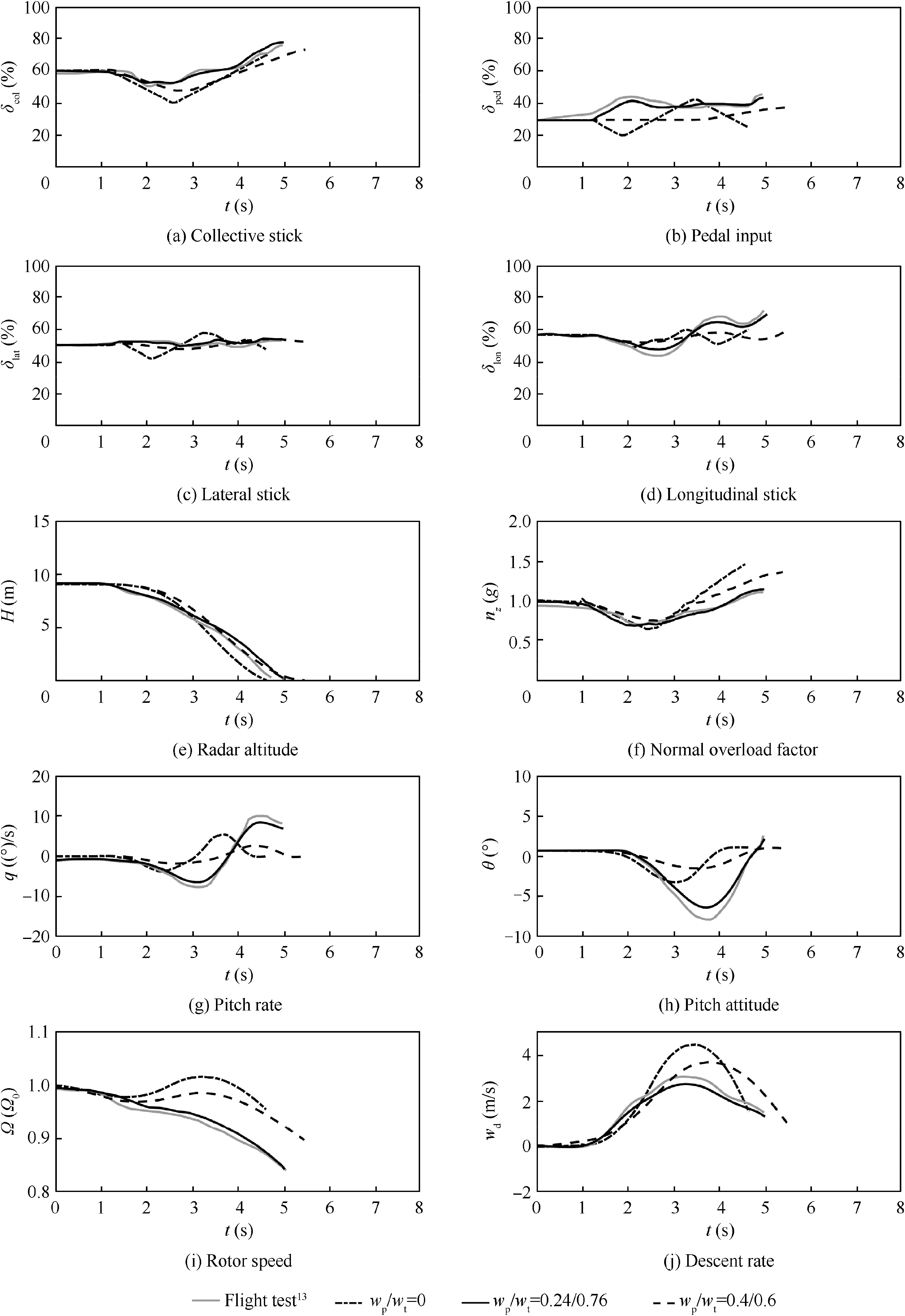
Fig. 4 Comparison of optimal solution and flight test data for safe landing in OEI.

The assignment of pilot workload weight coefficientwpand time weight coefficient wthas a great influence on the landing procedure.To determine a reasonable weight coefficient distribution,this section compares and analyzes the optimal landing trajectory and control strategy under different wp/wtin the performance index J.

As presented in Fig. 4, for the flight test data and the optimal solution under different wp/wt,the trend of control strategies in the longitudinal plane are basically close. Pilot first reduces the rotor collective pitch (Fig. 4(a)) to maintain the speed of rotor rotation and controls the longitudinal cyclic pitch (Fig. 4(d)) to make helicopter decline (Fig. 4(h)). Then,pilot increases the rotor collective pitch and the pitch attitude angle to reduce the descent rate and land safely. In addition,the pilot has to stabilize the attitude of helicopter through some small adjustments of lateral stick (Fig. 4(c)) and pedal controls (Fig. 4(b)).

Table 1 Constituent frequencies for control tasks.24

For the optimal solution, with the increase of the ratio wpto wt, the control strategy becomes smoother. When the performance index ignores the item of pilot workload(wp/wt=0), the control time required for landing is less than 5 s. However, the control strategy is quite intense for pilot,especially in pedal and lateral controls, which makes it necessary to add the pilot workload term in the performance index to decrease control difficulty.In addition,the variation amplitudes of descent rate (Fig. 4(j))as well as the normal overload factor (Fig. 4(f)) at touchdown are much larger than other results.

When wp/wtincreases to 0.24/0.76, the optimal control strategy is basically consistent with the pilot control input in the flight test, as well as the optimal landing trajectory, which indicates that the augmented model and optimal control method applied in this paper are feasible. Notice that in the real flight test,the data of control strategy and flight trajectory could be affected by some factors such as slight difference of the environment, and the physical state as well as the psychological state of the pilot. This paper mainly considers the parameter wp/wtin the performance index to make the simulation results close to the actual flight test. Therefore, the simulation results are not expected to be completely consistent with the real test data, but the results still indicate that the method really captures the main characteristics of the pilot control strategy and flight trajectory.

When the ratio wp/wtcontinues to increase to 0.4/0.6, the pilot controls are much smoother,but the variation of descent rate and the normal overload factor at touchdown will further increase.

6. Evaluation of pilot workload

This section analyzes and compares the pilot control activities and pilot workloads of the flight test13and the optimal solution under different wp/wtfor UH-60A helicopter landing procedure in OEI.

Pilot workload is a hypothetical construct that represents the cost incurred by pilot to achieve a particular flight task.Although there are many factors that will affect the pilot workload, including the flight environment, pilot skills, perception,experience and so on, the pilot workload is often estimated based on the time histories of the pilot control inputs.14,15,21,22Intuitively,the factors that primarily affect the pilot workload can be described as the amplitude and frequency for each pilot control input, and the complexity of the cooperation between them. Considering the limits of the pilot inherent characteristics, high frequency and large-scale operations as well as the excessively complicated cooperation between the pilot control inputs will obviously increase the pilot workload. In other words, low frequency and small amplitude of pilot controls with simple coupling of control inputs will help to reduce the pilot workload. In this paper, the pilot control activities are quantified and evaluated based on the pilot control inputs of the optimal solution and the flight test data in Fig.4.The pilot workloads are also compared and discussed.

Early attempts used a few simple metrics to analyze pilot control inputs, such as the aggressiveness and the average duration of stable maneuvers based on time domain.21More complex methods, such as Power Spectral Density (PSD) or Root Mean Square (RMS) of control inputs based on frequency domain, and the resulting cutoff frequency, are also used to describe or quantify the pilot workload.15,22,23However, these above analysis methods have inability to explain the temporal variation in pilot control strategy over the course of a maneuver, so such metrics may not provide a complete reference. To this end, a class of Time-Frequency Representation(TFR)based methods are used to analyze the pilot control activity such as time-varying cutoff frequency, power frequency, and multi-frequency. These TFR methods can be interpreted to provide unique insight into the PSD and the pilot cutoff frequency to account for the characterization of the way in which pilot control activity changes with time.14,15,23Among them, the time-varying cutoff frequency is basically similar in concept to the classical cutoff frequency,though it is computed from a TFR instead of a PSD. It provides a good estimate of the classical cutoff frequency over the course of the maneuver.The power frequency is computed by multiplying the time-varying cutoff frequency by the maximum signal power at that instant time.The multi-frequency is a TFR method based on short-time Fourier transform or wavelet analysis.It has the ability to identify the multiple constituent frequencies of pilot control activity at each instant time over the duration of maneuver. By comparison, the time-varying cutoff frequency and power frequency only describe a single frequency (or power frequency) at instant time,which is actually the result of combining the various constituent frequencies and magnitudes identified by the multifrequency method.

In fact, many researches14,15,23,24have shown that a pilot’s control input may simultaneously contain multiple constituent frequencies, which is important because the different frequencies are indicative of different piloting tasks or control strategies24(see Table 1).

By observing the description of the control strategies corresponding to the range of pilot’s constituent frequencies in Table 1, combined with the description of the Cooper-Harper’s Handling Quality Rating (HQR),22it can be found that there is a mapping relationship between the pilot’s constituent frequencies and pilot workload (see Table 2).

Therefore,the multi-frequency method can give a quantitative index of pilot workload with a simple HQR rating value.In addition, it is important to note that the frequency ranges and the control task descriptions in Table 1 are proposed for the pilot stick activity in fixed-wing aircraft.As such,the speci-fic descriptions are not expected to remain directly valid for the helicopter control inputs discussed here. Nevertheless, it still indicates that different frequencies correspond to different helicopter pilot control activities and pilot workloads.15

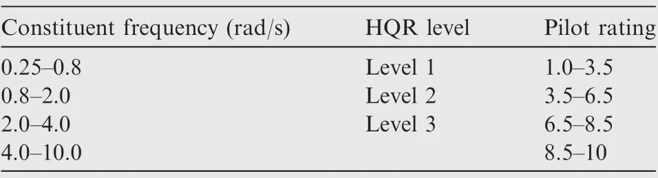
Table 2 Mapping relationship between pilot’s constituent frequencies and HQRs.

In all kinds of maneuvering tasks, the correlation between pilot low-frequency and high-frequency maneuvering is relatively high, and the measurement may contain the influence of noise, so the characteristics of signal are usually irregular.Thus the wavelet function suitable for pilot workload evaluation should have orthogonality, tight support set, good regularity, and moderate vanishing order. This paper chooses the db3 wavelet function25,26to perform the wavelet analysis of pilot control activity.

After determining the wavelet function, the pilot control inputs (time-varying signal) can be wavelet transformed. The wavelet function is scaled by scaling factor s and translated by parameter u. The scaling factor corresponds to frequency and the translation parameter corresponds to time. Then the wavelet function and its Fourier transform can be expressed as

where Wy（u ，s）is called the wavelet coefficient and*represents the conjugate relationship. The modulus (magnitude) of Wycan reflect the distribution of energy for pilot input signal δ（t ） with time and frequency in the TFR.

Fig. 5 shows the TFRs of pilot collective control activities based on the flight test and the optimal solutions under different values of wp/wt.

The TFR of collective control activity from the flight test is shown in Fig. 5(a). It can be found that there are two distinct magnitude peaks at around 2.5 s and 4.5 s, the corresponding constituent frequencies are 1.0-1.6 rad/s and 1.0-2.0 rad/s,where the former magnitude is less than the latter. These two peaks correspond to the pilot’s reduction of collective control to maintain the speed of rotor rotation at first,and the increase of collective control to land safely at last.In addition,there are some constituent frequencies higher than 2.0 rad/s, but the magnitudes are extremely low, which corresponds to the pilot small manipulation.

The TFR of collective control activity from the optimal solution are shown in Fig. 5(b)-(d) for different values of wp/wt. It can be found that for the case of wp/wt= 0.24/0.76, the variation of constituent frequencies and corresponding magnitudes with time is very close to that of the flight test as shown in Fig. 5(c). For wp/wt= 0 (no consideration of pilot workload), the variation of constituent frequencies with time is basically close to that of the flight test. However, the magnitude at 2.5 s is too high (larger pilot manipulation) and the magnitude at 4.5 s is too low compared with those of flight test. For the case of wp/wt= 0.4/0.6, the result is similar with that of wp/wt= 0 although the magnitude and the constituent frequencies are better.

Fig. 6 shows the TFRs of pilot lateral control activities based on the flight test and the optimal solutions under different values of wp/wt.It can be seen that the magnitudes in Fig.6 are very low compared with the magnitudes in Fig. 5, indicating that the pilot lateral controls are very small compared with the collective manipulation.

For the TFR of lateral control input from the flight test in Fig.6(a),there are two distinct magnitude peaks at around 2 s and 3.5 s, and the corresponding constituent frequencies are 1.8-2.0 rad/s and 2.0 rad/s,where the former magnitude is larger than the latter.In addition,there are some constituent frequencies higher than 2.0 rad/s, but the magnitudes are low,which can be ignored.

For the TFR of lateral control input from the optimal solutions with every value of wp/wtshown in Fig.6(b)-(d),the distribution of the magnitude peaks and the corresponding constituent frequencies are different from those in Fig. 6(a).The reason is that the lateral control is very small and the measurement error may exist in the data acquisition of pilot’s lateral manipulation in the flight test. In practice, the pilot’s lateral manipulation is always small during the helicopter landing after one engine failure, and the lateral operation process has no effect on the safe landing.

Fig. 7 shows the TFRs of pilot longitudinal control inputs of the flight test and the optimal solutions under different values of wp/wt. For the TFR of longitudinal control input from the flight test shown in Fig.7(a),there are two distinct magnitude peaks at around 2.5 s and 4 s,and the corresponding constituent frequencies are 1.5-1.8 rad/s and 1.8 rad/s. These two peaks correspond to the pilot control process of helicopter head-down acceleration and head-up deceleration landing. In addition,there are some high-frequency components at around 2.7 s, 3.6 s and 5 s, but the magnitudes are low.

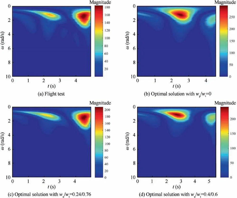
Fig. 5 TFRs of pilot collective control inputs of flight test13 and optimal solution.

Fig. 6 TFRs of pilot lateral control inputs of flight test13 and optimal solution.

Fig. 7 TFRs of pilot longitudinal control inputs of flight test13 and optimal solution.

Fig. 8 TFRs of pilot pedal control inputs of flight test13 and optimal solution.

For the TFR of longitudinal control input from the optimal solution with wp/wt= 0 (no consideration of pilot workload)in Fig.7(b), the maximum magnitude is much lower than that of flight test, and there are many high-frequency components distributed in 2.0-10.0 rad/s, indicating a higher pilot workload with urgent control.When wp/wt= 0.24/0.76,the wavelet transform result is very close to that of the flight test.When the ratio wp/wtcontinues to increase to 0.4/0.6,the magnitudes and the high-frequency components are further reduced. It is noted that although the magnitudes are small when wp/wt= 0 and 0.4/0.6 (i.e. small longitudinal control), it can be seen from Fig. 4 that the variation of descent rate and the normal overload factor at touchdown will increase.

Fig. 8 shows the TFRs of pilot pedal control activities of the flight test and the optimal solutions under different wp/wt.For the TFR of pedal control input from the flight test shown in Fig.8(a),there is a wide range of low constituent frequency (0.5 rad/s) throughout the landing procedure, which corresponds to the pilot control process of trimming and flight path modulation.

For the TFR of pedal control input from the optimal solution with wp/wt= 0 (no consideration of pilot workload)shown in Fig.8(b),the maximum magnitude is lower than that of flight test.But there are two distinct peaks at around 2 s and 3.5 s, the corresponding constituent frequencies are 1.8-2.0 rad/s and 2.0 rad/s, and the high-frequency components are more obvious, indicating a maneuvering control process with more urgency. When wp/wt= 0.24/0.76, the wavelet transform result is almost identical with that of the flight test,and the high-frequency component at 3.5 s has disappeared,which is obvious in Fig. 8(b). When the ratio wp/wtcontinues to increase to 0.4/0.6, the maximum magnitude is greatly reduced, and a low constituent frequency (1.0-2.0 rad/s)appears at the end, which corresponds to the pilot control of yaw angle adjustment at touchdown.

For all the TFRs of pilot control inputs,the wavelet transform results are very close to those of the flight test when wp/wt= 0.24/0.76. It indicates that the pilot workload can be evaluated during the helicopter landing after one engine failure. The Cooper-Harper HQR assigned by the pilot in the flight test is HQR 4-5 in Level 2,13hence the pilot workload in the optimal solution with wp/wt= 0.24/0.76 can also be evaluated as around HQR 4-5 in Level 2.

It is important to notice that the parameter wp/wtin performance index J may be different in other OEI cases. It is dependent on different OEI conditions and control characteristics of different pilots. Nevertheless, the results in this paper still indicate that the optimal control method and the wavelet analysis method of pilot control activity provide a tool to predict the pilot workload in helicopter landing after one engine failure.

7. Conclusions

This paper provides a method that can be used to evaluate the pilot workload of helicopter landing after one engine failure. The UH-60A helicopter is taken as the example. Based on an augmented six-degree-of-freedom rigid-body flight dynamics model, the optimal landing procedure is formulated as a nonlinear optimal control problem in the form of performance index, path constraints and boundary conditions,solved by collocation and numerical optimization method.A time-frequency domain method called wavelet analysis is utilized to quantify and evaluate the pilot activity and pilot workload. The optimal landing trajectory and controls are compared with those from the flight test data, and the pilot workloads based on the pilot control inputs of the optimal solution and the flight test data are also compared and discussed. Based on the results obtained, the following conclusions can be drawn:

(1) When the performance index ignores the item of pilot workload, the control strategy is quite intense for the pilot, especially in pedal and lateral controls, and the variation amplitudes of descent rate as well as the normal overload factor at touchdown are much larger than other results.When the performance index considers the factor of pilot workload, the optimal control strategy is basically consistent with the pilot control inputs in the flight test, as well as the optimal landing trajectory,which indicates that the augmented model and optimal control method applied in this paper are feasible. When the proportion of pilot workload item continues to rise,the pilot controls are much smoother,but the variations of descent rate and the normal overload factor at touchdown will further increase.

(2) The TFRs show that the helicopter landing task in OEI from Ref. 13 belongs to conventional maneuvering with small urgency. When the performance index considers the factor of pilot workload,the characteristics of amplitude and constituent frequencies of pilot control inputs in the optimal solution are basically consistent with those of the pilot control inputs in the flight test. It can be concluded that the pilot workload evaluated in this paper is basically consistent with that of the flight test. The Cooper-Harper HQR assigned by the pilot in the flight test is HQR 4-5 in Level 2, hence the pilot workload in the optimal solution can also be evaluated as around HQR 4-5 in Level 2.

(3) Based on the analysis of time history and TFRs of pilot control inputs in the flight test data and the optimal solution,it is reasonable to believe that the optimal control method and the wavelet analysis method of pilot control activity provide a tool to predict the pilot workload in helicopter landing after one engine failure.

Acknowledgment

This work was supported by the National Natural Science Foundation of China (No. 11672128).