Effects of Mach numbers on Magnus induced surface pressure
2020-02-24ASKARYSOLTANI
F. ASKARY, M.R. SOLTANI
a Department of Aerospace Engineering, Sharif University, Tehran P.O.B 1458889694, Iran
b Department of Aeronautics and Astronautics, University of Washington, Seattle BOX 352400, USA
KEYWORDS Magnus effect;Spinning projectile;Surface pressure;Wind tunnel
Abstract Experimental and numerical methods were used to investigate the Magnus phenomena over a spinning projectile.The pressure force acting on the surface of a spinning projectile was measured for various cases by employing a relatively novel experimental technique. A set of miniature pressure sensors along with a data acquisition board, battery and storage memory were placed inside a spinning model and the surface pressure were obtained through a remotely controlled system.Circumferential pressures of the model for both rotational and static conditions were obtained at two different free stream Mach numbers of 0.4 and 0.8 and at different angles of attack. The results showed the ability of this new test method to measure the very small Magnus force via surface pressures over the projectile.The results provide a deep insight into the flow structure and illustrate changes in the cross-flow separation locations as a result of rotation. Similar results were obtained by the numerical simulations and were compared with the experimental data.
1. Introduction
A spinning projectile experiences surface pressure variation that results in the so-called Magnus effect. This external aerodynamic phenomenon, which is caused by combinations of projectile rotation and angles of attack,provides a corresponding forces and moment that can destabilize the projectile during its flight.1,2The Magnus force is very small relative to the normal force; however, it may significantly affect the range and accuracy of the projectile.3
Magnus forces and moments acting on the rotating projectiles create a very complex flow feature around them.Exclusive experimental and theoretically studies have been undertaken to realize the fundamental Magnus phenomena and to better explain the physical feature of the undesired effects. At low to moderate rotational speeds and at small angles of attack,the boundary layer on the surface of the projectile remains attached,hence the Magnus effect is mainly due to interaction of the potential flow with the asymmetric boundary layer around the circumference of the body.The concept of circulation, common in the circular cylinder analysis, has only recently been mentioned in a few analytical approaches.4-6At higher angles of attack, the flowfield over the projectile behave similar to that of the circular cylinder placed in the cross flow.7,8
Nomenclature
N Normal force
YMYawing moment
SFSide force
CmPitchnig moment coefficient
CnYawing moment coefficient
CNNormal force coefficient
CYSide force coefficient
Cyp∂CY/∂(pd/2V)
Cnp∂Cm/∂(pd/2V)
CpPressure coefficient
ΔCpVariation of Cpdue to spin
d Body diameter
p Spin rat
P Tip speed ratio
l Projectile length
S Reference area
V∞Free stream velocity
V∞nNormal component of freestream velocity
Ma∞Free stream Mach number
q∞Free stream dynamic pressure
α Angle of attack
Φ Circumferential location
Re Reynolds number
x, y, z body axis
For a spinning projectile at angles of attack, however, the flow field over the body depends on many factors, the angles of attack, the speed of rotation, and the Reynolds number which affect the status of the boundary layer as well as the separation of the lee side vortices, etc. At small angles of attack,the flow remains attached and the lee side vortices are embedded in the boundary layer.For both low Reynolds number and spin rates, the boundary layer remains laminar and skewed in the direction of the rotation.The boundary layer becomes turbulent at higher Reynolds numbers.9,10
For very high angles of attack, but at both small spin rates and low Reynolds numbers, the vortices become separated from the body; however, the boundary layer remains laminar.For most projectiles where the flow separates at a relatively small angles of attack, about five degrees or so, it has been noticed that spin rate has significant effects on the separated vortex sheets. At high angles of attack the Magnus forces become negative and the vortex contribution dominates the entire flowfield.11
Almost all of the existing theories that try to predict effects of the Magnus forces have practical limitations. Although some insight such as the way in which the Magnus force shows itself is gained from these analytical methods, the existing approaches cannot yet be used to predict various features of the flowfield involved when the projectile is spinning or operating at high angles of attack. Therefore, the main source of the Magnus data is from the conventional wind tunnel tests.The ability to measure the forces is prevented by the fact that the Magnus force is at least an order of magnitude smaller than the existing normal force, which provides a challenge for the experimentalists to implement schemes capable of measuring this small force and its variations with spin, angles of attack, Reynolds number, etc.
Most of the wind tunnel balance systems currently used for measuring the aerodynamic loads of a spinning projectile is of the type shown in Fig. 1. This mechanism consists of an airturbine-driven model that is mounted on the bearings with an internal strain gauge balance. Due to the very high spin rates of the projectiles,both model design and dynamic balancing become an integral and important part of the experiment.
The sources of errors involved in such measurements are attributed to the model-induced oscillations due to the free stream turbulence, test section Mach number variations, tunnel flow angularity,etc.In general,the measured motion from the free flight tests is curve fit analytically in a least squares sense and a quasi-linear model of the motion is obtained.The models derived from this technique are usually considered of the tricyclic or a quadricyclic theory form, and both frequencies and damping obtained from the fitted data are used to predict the corresponding aerodynamics, including the Magnus terms.12,13
Over the past few years, the circumferential pressures around the spinning projectiles have been measured using a non-conventional model and instrumentation arrangements.For almost all cases studied, the models were made up of two parts, a non-rotating internal section housed inside an outer rotating model. The necessary instrumentations used to detect the surface pressures were housed inside the nonrotating portion of the model at various locations. A series of pressure ports were drilled around the outer spinning portion of the model and the pressure for each port was measured using a sliding seal arrangement.14The reliability as well as the performance capability of this testing technique has been demonstrated with a simple spinning circular cylinder, however, the versatility and accuracy of this method is questionable when using the unconventional models.15Other researchers have tried to improve several elements of the instrumentation, in particular the critical sliding seal units.This latter work evolved with a miniature sized seal and a remotely selectable pneumatic magnetic fluid seal (to reduce the friction effects); all intended to increase the reliability and accuracy of the measurement techniques.16

Fig. 1 Wind tunnel balance system.
Recent developments of electronic devices and sensors have made it possible for the experimentalists to conduct wind tunnel tests on the spinning projectiles for situations similar to their flight conditions. This is done by using very small pressure sensors, Wi-Fi connectivity, miniature accelerometers,where all of them can easily be placed inside a small model used for small wind tunnels.
This paper presents a novel method for measuring the surface pressure of a spinning projectile in a wind tunnel under different conditions. The model consists of an ogive, cylinder and boattail. The model has a length of 33 cm and a diameter of 7.7 cm and was tested in a trisonic wind tunnel. Circumferential pressures were obtained at several longitudinal locations on the model with special emphasize on the boattail section.The model was tested at angles of attack of α=0, 5, 10, 15,20 and 25 degrees and at a rotation rate of 5000 r/min.All tests were performed at two free stream Mach numbers of Ma∞=0.4 and Ma∞=0.8. In addition, the aerodynamic forces and moments of the model for the static case,zero spin,were obtained from an internal strain gauge-balance system.The static surface pressure distributions were measured for both rotating and non-rotating condition.
The test described in this paper is intended to illustrate the capability and accuracy of a new method of measuring the surface pressure distribution over a spinning projectile, which to the author’s knowledge, has not been done before or if it has been done previously,the method and the results are not publicly available. The experimental data are used to support the evolution and validation of the existing theoretical and numerical analyses and allows a detailed insight into the Magnus phenomena. In addition, the results demonstrated that this new technique could provide the pressure data on a rotating projectile accurately with any desired spin rate.
As mentioned, to make sure that the flow undergoes from the attached to the separated phases over the boattail part of the model, the angles of attack of the model were varied from 5 to 25 degrees.As a result,the aerodynamic characteristics of the model will be significantly different and the resulting pressure signature would be of extreme interest.The present newly designed mechanism can rotate a model weighing up to 5 kg with an adjustable rotational speed from zero to 5000 r/min.The selected rotational speed of 5000 r/min represents a tip speed ratio of 0.16 and 0.08 corresponding to the free stream Mach numbers of Ma∞=0.4 and Ma∞=0.8 respectively.In this paper, however, the data for Ma∞=0.8 is compared with those of Ma∞=0.4 and the effect of varying free stream Mach number on the surface pressure data on the corresponding Magnus force and moment is discussed.
2. Wind tunnel and instrumentation
The wind tunnel used in these experiments is of an open circuit suction type with a rectangular 60×60 cm2test section. This tunnel can continuously work for a variety of Mach numbers,Ma∞=0.4-2.5, without any restrictions on the run time.17The turbulence intensity in the test section varies from 0.41% to 1.42% for Reynolds number of 6.37×10⁶to 7×10⁷per meter. The free stream Mach number is obtained by a variable nozzle and jet engines.The maximum flow angularity in the test section is reported to be less than 0.5°.18
3. Model description
A schematic drawing of the internal arrangement of the model is shown in Fig. 2. It consists of a 12 cm ogive nose, a 10 cm cylinder, and a 11 cm boattail. The total length of the model is 33 cm and the maximum diameter is 7.7 cm. The model is equipped with 11 pressure ports along its length. All pressure ports have 0.8 mm diameter and are used to measure the surface static pressure at various testing conditions. The model is attached to a servo motor through a bearing mechanism. The servo motor provides the required rotational speed. The maximum variation of the rotation of the model was measured to be less than 1.5 r/min for each specified rotational speed.
A 16-bit,16 channels data acquisition board,an 8 Gigabyte storage memory, a rechargeable li-ion battery and a Wi-Fi connection were placed inside, at the center of the model via three miniature rings. All pressure ports were connected to the miniature pressure sensors through thin steel tubes with a maximum length of less than 5 cm. In the center of the data acquisition board, a 3-axis accelerometer sensor is placed that senses the gravitational acceleration from which the circumferential positions of the pressure ports when the models is spinning were accurately determined. The output of the accelerometer was synchronized with the data of the miniature pressure sensors. Data for all ports were collected simultaneously.
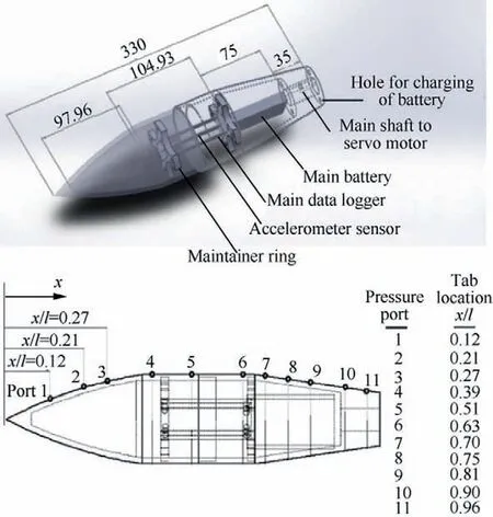
Fig. 2 Schematic of internal parts of model and location of longitudinal pressure ports.
The test procedure was to first establish the tunnel air flow at the desired Mach number. The model was then set to the desired angle of attack and spun-up to the specified spin rate after which the data acquisition through a command from the computer was started. The acquired data were stored in a storage memory located on the data acquisition board inside the model and were transferred to the computer through a Wi-Fi connection simultaneously or later at a leisure time.
The pressure sensors were of high-frequency miniature ones and were positioned inside the model as close as possible to the pressure ports to ensure minimum time lag. These miniature transducers were used to measure both steady and unsteady surface pressure.19The sensors were of differential-type pressure transducers with a maximum combined nonlinearity,repeatability and hysteresis of about 0.5% of their full-scale output.
A small pre-pressurized tank was placed inside the model to ensure that all of the miniature pressure sensors have the same reference pressure value. For each angle of attack, the data from all transducers and other equipment were acquired with a frequency of 5 kHz for 15 s and the model was spinned about 1250 times while the circumferential pressures at 11 longitudinal locations were recorded simultaneously.The instantaneous circumferential angle of the model for each cycle was calculated from the output of the three-axis accelerometer sensor placed inside the model. All data were low pass filtered and the final pressures at all stations, 11 of them, were obtained through superposition of the circumferential pressure cycles.
The present wind tunnel tests are carried out at angles of attacks from zero to 25° and at zero degrees side slip angle for two free stream Mach numbers of Ma∞=0.4 and Ma∞=0.8.Fig.3 shows the model installed inside the tunnel test section as well as the rotational mechanism.The measured surface pressure data for each condition were then reduced to coefficient form as defined in Fig. 4.
4. Numerical methodology
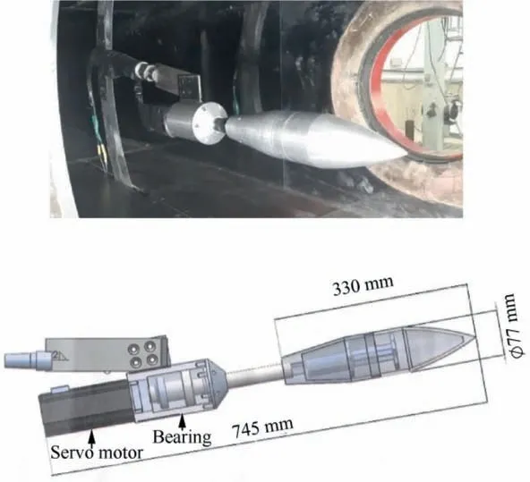
Fig. 3 Model and spinning mechanism.

Fig. 4 Definition of various terms used in the paper.
The same projectile was modeled for the numerical simulation.The projectile model in the wind tunnel and the computational grids are shown in Fig. 5. The simulations were performed on an unstructured grid with triangular prisms in the boundary layer and with tetrahedral ones elsewhere. The grid has approximately 1.7×10⁶cells which was chosen after a rigorous grid independence study.
A cylindrical zone was created around the projectile where its axis was coincident with the body axis.The grid was refined within this cylinder to completely capture the vortices over the leeward side of the projectile.The projectile and the cylindrical zone were rotated as a solid body. The cylinder surface was coincident with another cylindrical surface which was fixed and belonged to the rest of the domain.With a‘‘sliding mesh”approach there is no need for the time-consuming methods like remeshing or a spring mesh motion.
To accurately simulate the flow structure, a grid study was performed by checking the convergence of the numerical values of the flow field variables at several flow field locations.An example is shown in Table 1 which shows the average non-dimensional axial and tangential velocities (u/V∞, v/V∞)in a selected point near the leeward portion of the projectile at the junction of boattail and cylindrical section at Ma∞=0.8. The grid has a first wall spacing of y+=20 which is appropriate for the turbulent model used in this study.The surfaces of the wind tunnel test section walls and the projectile were specified as the solid wall with no-slip boundary conditions.Both the inlet and the outlet of the wind tunnel test section were considered as the pressure inlet and the pressure outlet boundary conditions respectively.
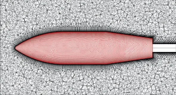
Fig. 5 Computational grid around projectile.

Table 1 Axial and tangential velocity component for various grid sizes at an arbitrary point.
The three-dimensional unsteady compressible Navier-Stokes equations were solved as the governing equations.The upwind MUSCL algorithm was applied to extend the spatial accuracy to the 2nd order based on the primitive variables and the numerical fluxes for the convective terms were computed using Roe’s scheme. The two equations SST k-ω turbulence model was applied and the entire flow field was assumed to be fully turbulent. The viscous fluxes were computed using the 2nd order central differencing scheme. Different versions of the k-ω turbulent model have been found to be appropriate to capture the flow field over the rotating body by several researchers.20For the unsteady time integration an implicit dual-time algorithm was applied. The viscosity was calculated by the Sutherland’s law and the density was calculated by the ideal gas law.A valid CFD code was available for the researchers with the aforementioned capabilities and several conditions were selected to be simulated numerically.
5. Results and discussion
The circumferential pressure distribution at various longitudinal locations over the surface of the projectile for different angles of attacks and for two different free-stream Mach numbers is studied. These data illustrate the capability of the new testing technique to measure both steady and transient pressure variations accurately for different conditions along the surface of the model. The pressure sensors were capable of measuring pressure differences as low as 35 Pa.Data for these tests show excellent repeatability for all cases examined in this investigation. The uncertainties of the measured ‘‘Cp” for this study are calculated and estimated to be less than 0.54%of the full scale.


Fig. 6 Output of one of pressure sensors, α=5°, Ma∞=0.4.

Fig. 7 Circumferential pressure distribution at two longitudinal stations, α=5°, Ma∞=0.8.
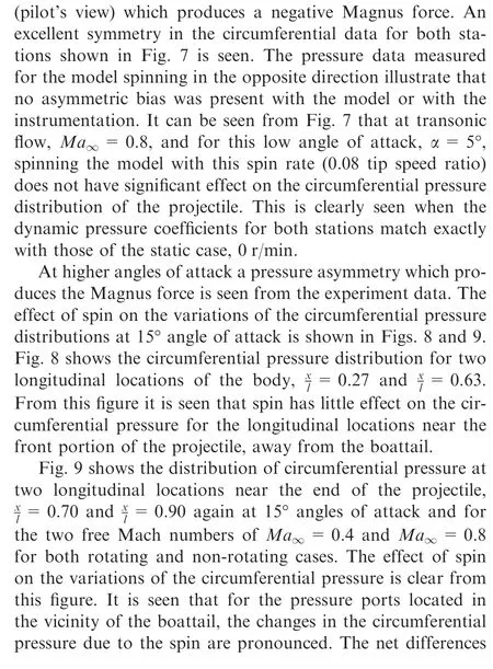


Fig. 8 Circumferential pressure distribution in vicinity of nose and midsection, α=15°.
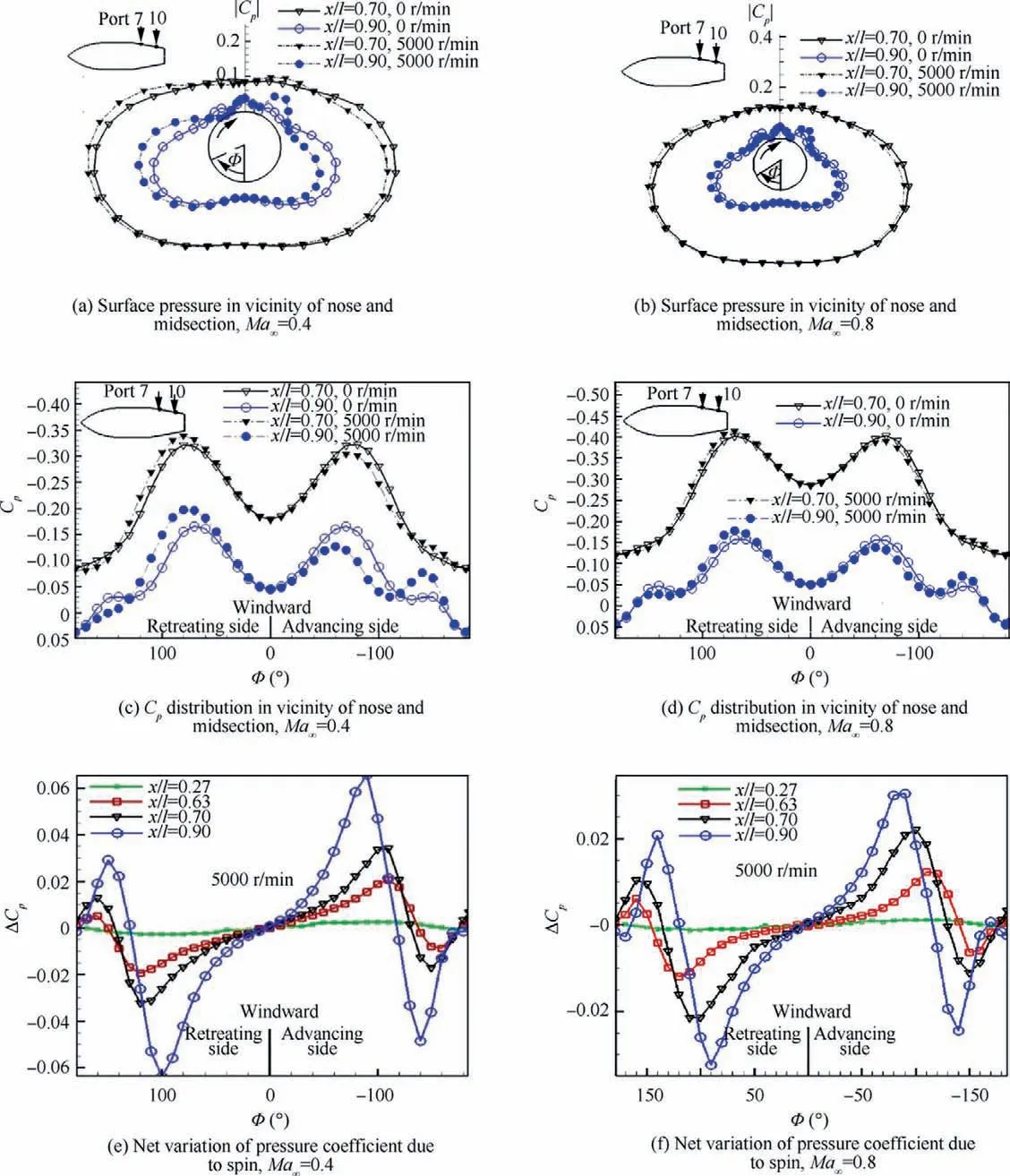
Fig. 9 Circumferential pressure distribution at two longitudinal stations, α=15°.

Fig. 10 Circumferential pressure distribution at two longitudinal stations, Ma∞=0.8, α=25°.

Fig. 11 Effect of angles of attack on circumferential pressure distribution at various longitudinal stations, Ma∞=0.8.
The net variations of the pressure coefficient at four longitudinal locations due to the spin at 25°angle of attack is shown in Fig. 10(c). This data illustrates presence of a negative pressure on the retreating side of the windward portion of the projectile(Φ ≈10°to 100°)followed by a positive pressure due to the spin on the same side of the leeward portion of the projectile (Φ ≈120° to 160°). The ΔCpvalues for the positive and negative pressure due to rotation is larger for the pressure port
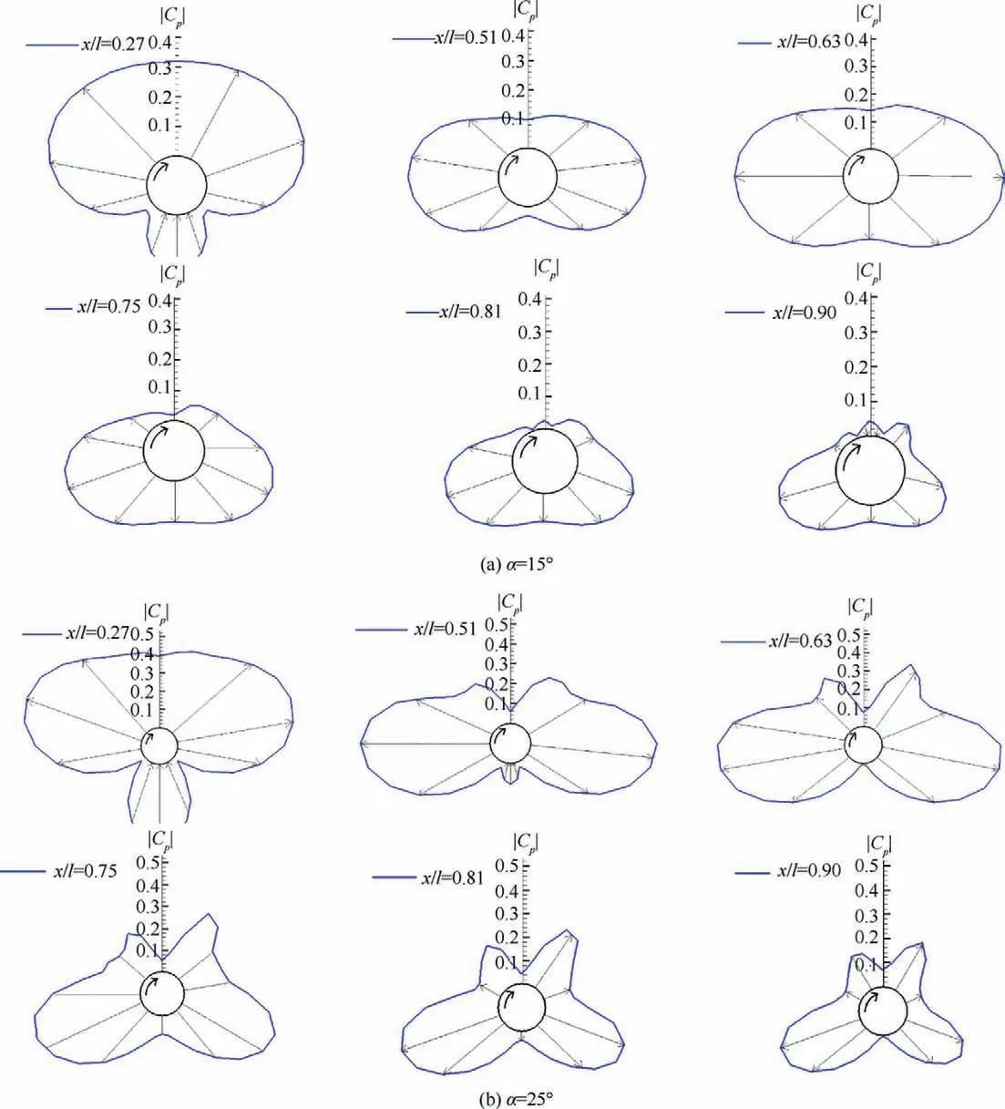
Fig. 12 Circumferential surface pressure distribution on spinning projectile, Ma∞=0.8, p=5000 r/min.
located in the vicinity of the boattail,>0.63. Moreover, a positive pressure on the advancing side of the windward portion of the projectile (Φ ≈-20° to -100°) followed by a negative pressure due to spin on the leeward portion of the projectile (Φ ≈-130° to -155°) are seen from Fig. 10(a)-(c).Similar and greater changes in the circumferential pressure induced by rotation were observed at a free-stream Mach number of Ma∞=0.4.


Fig. 13 Comparison of surface pressure distribution obtained by CFD and wind tunnel test on spinning projectile, Ma∞=0.8.

In the experimental tests performed in this study, only the circumferential pressure distribution on the model surface was measured.With respect to the circumferential pressure distribution, the presence of vortices formed over the leeside of the projectile,especially at locations near the end of the model,are vividly seen at high angles of attack.The existence of these vortices and their presence are further verified by the numerical studies for the same model at the same conditions.
Fig.13 compares both numerical and experimental circumferential pressure coefficient results on the rotating projectile at two longitudinal stations for different flow conditions.In general, good agreement is achieved between the numerical and the present experimental results, especially for locations near the front of the projectile.In the leeward portion of the model by increasing the angle of attack the minimum pressure predicted by the numerical solution is slightly lower than that obtained by the experimental results. This difference becomes more vivid on the side of the projectile (Φ ≈±100°). On the leeward portion of the projectile, the difference between the numerical and the experimental results is seen to be relatively high (|Φ|>130°). This difference is expected because of the complex and random nature of the vortex region. In general,it can be concluded that dynamic results predicted by the numerical simulations are relatively reliable for portions of the model where flow asymmetry is not dominant and as a result the corresponding Magnus force and moment is negligible.

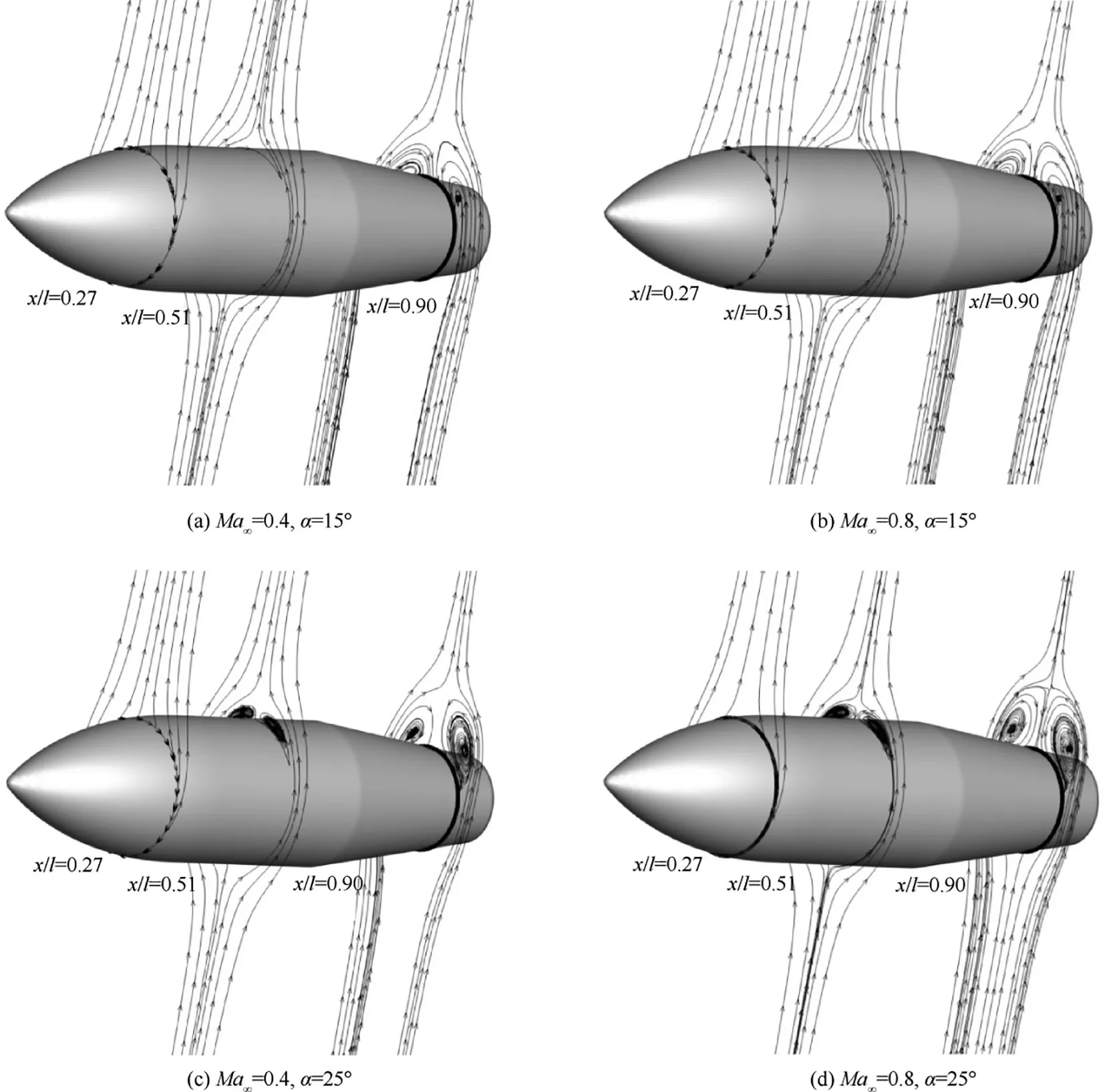
Fig. 14 Streamlines around projectile at several longitudinal locations for different flow conditions.

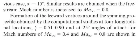
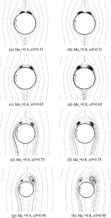
Fig. 15 Formation of leeside vortices at two longitudinal locations, α=25°, p=5000 r/min.
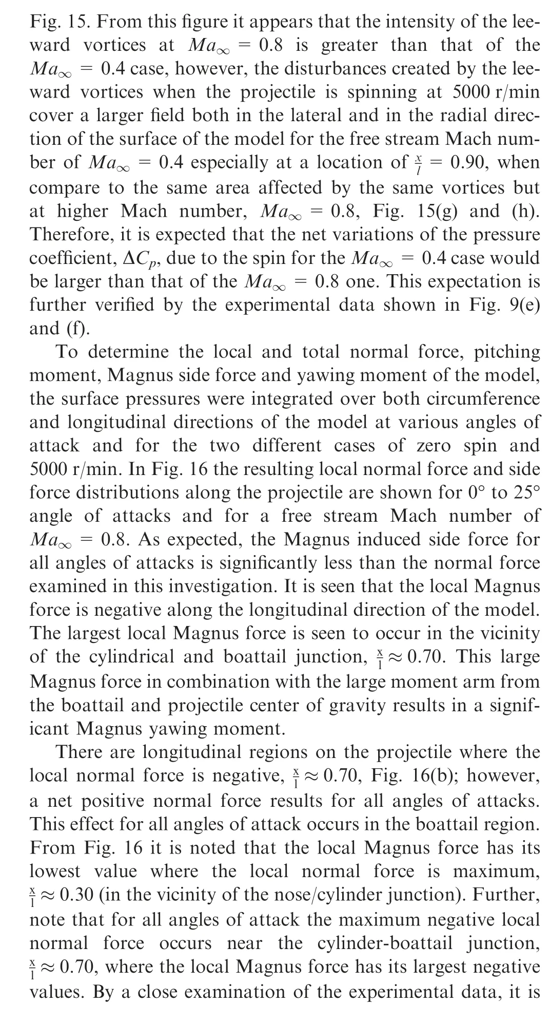
The normal force acting on the model was directly measured by a separate series of wind tunnel tests using a six component internal strain gauge balance. All tests were conducted with the same model and at the same tunnel conditions that the pressure measurement tests were conducted. Fig. 17 compares the normal force coefficient obtainedby integrating the surface pressure data over the circumference and then over the length of the model with the measured balance data at different angles of attacks. Note that the CNdata are obtained from integration of only 11 longitudinal pressure ports located on the projectile surface,Fig.2.Therefore;one expects that there will be differences in all force and moment calculation obtained by integrating the limited pressure signatures from those measured by the balance or from the computational result.
The maximum normal force obtained from the pressure distribution at Ma∞= 0.4 is about 17% and at Ma∞=0.8 is about 20% lower than the normal force obtained from the wind tunnel balance system. The difference between the normal force coefficients from the balance and surface pressure integration are due to the limited number of pressure ports on the model. As stated in the paper there were only 11 pressure ports on the model that causes the pressure distribution on the model for integrating to be discontinuous.Note the limited number of pressure ports were mainly due to the available high response pressure transducers. On the other hand, the balance system measures the overall forces and moments.Although the dominant share in the calculation of the normal forces belongs to the pressure forces, however, viscous forces have their own share too. Overall, the trend of variation of all forces and moments from both measuring technique, balance and surface pressure integration are the same.Moreover,the balance data does not show variations of local forces and moments, while, the pressure data provides an in-depth inside into the origin of the variations as seen from the pressure data provided in this paper.
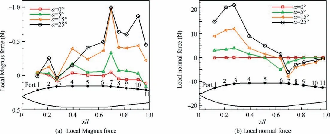
Fig. 16 Local Magnus and normal force distribution on spinning model, Ma∞=0.8, p=5000 r/min.

Fig. 17 Effect of Mach numbers on variation of normal force coefficient.

Fig. 18 Effect of Mach numbers on variation of Magnus force coefficient.
The data are also compared with the CFD results. From this figure it is noticed that the trend of CNvariations with angles of attack for all three methods are similar.The effect of Mach number on the CNvariation using both balance and surface pressure data shown in this figure is seen to be negligible for low angles of attack, α ≤10°, while at higher alpha the effect seems to be significant. Note that for the free-stream Mach number of Ma∞=0.8,it is expected that at high angles of attack the flow may become supersonic, over a portion of the model, terminating with a shock wave at the end of the boattail which will affect the boundary layer over the surface of the projectile.From Fig.17 note that CNvaries linearly with angels of attack for both Mach numbers examined here up to α ≈10°. For angles of attack larger than 10°, variation of the static CNwith alpha become nonlinear,Fig.17.The flow over the projectile for these angles of attack, α>10° is similar to that of a delta wing model where a pair of leading-edge vortices form over the surface of the model and their behavior dominate the lifting mechanism. As soon as these vortices form, variation of the aerodynamic force and moments with angles of attack become nonlinear, as seen from Fig.17.Variation of the Magnus force coefficients, Cyp, and the Magnus yawing moment coefficient, Cnpwith angle of attack for both Mach number, Ma∞=0.4 and Ma∞=0.8 and for 5000 r/min are shown in Fig. 18. The results from CFD calculations are shown for comparison too. As mentioned before, the present balance set-up cannot be used when the model is spinning.The calculated Cypand Cnpdata from the surface pressures as explained before, compares very well with those obtained by the CFD results for the same conditions. Fig. 18 shows that the Magnus force coefficient varies slightly with Mach number and its absolute value decreases as the free stream Mach number is increased from Ma∞=0.4 to Ma∞=0.8.However,the Magnus moment coefficient, Cnp, is seen to be greater at Ma∞=0.4 relative to Ma∞=0.8. Moreover, from Fig. 18 it is seem that the slopes of both Cypand Cnpfrom 0° to 5°angles of attack are not the same as thesis slopes from 5° to 25°. However for both range of angles of attacks,0°≤α ≤5° and 5°≤α ≤25°, both Cypand Cnpare seen to vary linearly with angles of attack.
As a concrete conclusion, it can be said that spinning the model at Mach number 0.8 generates much more Magnus force than that obtained at Mach number 0.4 at angles of attack up to 20°. The increase in the force of Magnus force is at least 200% at lower angles of attack such, i.e., 5° and 10°. This is well illustrated in Fig. 18(c). However, at high angles of attack, α>20°, the trend is seen to be reversed.
6. Conclusions
A new testing technique to study the surface pressure distribution over a rotating projectile in a wind tunnel has been developed and satisfactory results are obtained. Integration of the resulting pressure distribution over the surface of the model provides a quantitative measure of the aerodynamic forces such as the normal and the Magnus forces.Changes in the circumferential pressure at various angles of attack allow interpretation of the Magnus force created during the spinning process. The results provide a deep insight into the flow structure and illustrate changes in the cross-flow separation lines as a result of the spin. The simplicity along with the relative versatility of the method makes it applicable to a wide range of wind tunnel investigations during the rotation of the model.
The static, zero spin normal force coefficient was also obtained directly from the internal strain gauge balance during the tests. In addition the normal force coefficient is computed from integrating the measured surface pressure data and good agreement with the measured balance force data for similar situation, zero spin, is achieved.
At low angles of attack,rotation causes a weak asymmetry of the boundary layer profile. The circumferential pressure indicates existence of the leeward vortices at high angles of attack. At high angles of attack,rotation causes the separated vortex sheets to be altered and become asymmetric.The vortex asymmetry generates additional lateral force that gives additional vortex contribution to the total Magnus effect. The occurrence of the secondary vortices at high angles of attack is presented as an explanation for the negative locally Magnus force acting on the projectile.The results showed that rotation has more effect on the circumferential pressure on regions close to the boattail portion of the model, while the effect is of less significant for regions near the nose of the projectile.Due to spin,a significant positive pressure region was detected on the advancing side of the projectile at longitudinal stations close to the boattail section of the model on the windward portion for all angles of attack while a weaker negative pressure region was detected on the advancing side on the leeward portion of the projectile.However,on the retreating side,opposite of the advancing side of the model,a significant negative pressure region was detected on the windward portion for all angles of attacks and a weaker positive pressure region was seen on the leeward portion.
Quantitative pressure data indicated contribution of the various projectile sections (i.e. nose, cylinder, boattail) to the Magnus effect. The data indicated influences of both spin and angles of attack on the Magnus force and revealed that for any condition,all portions of the projectile experience negative local Magnus force, however, different portions of the projectile can experience both positive and negative local normal force. At a free stream Mach number of Ma∞=0.4 the largest local Magnus force is generated at the end of the projectile, while at Ma∞=0.8, the largest local Magnus force occurs in the vicinity of the cylindrical and boattail sections of the model.Integration of the acquired pressure distribution provided a quantitative measure of the Magnus force as well as interpretation of the boundary layer and flow separation effects.
Near the boattail (at the junction of the cylindrical and boattail) a significant Magnus side force is produced for all angles of attacks. At this location, the normal force has its minimum value.At both Mach numbers,the smallest Magnus force occurs near the junction of the nose and the cylindrical portions where the largest local normal force occurs.
Although the present initial feasibility model was for a simple spinning projectile, the basic technique could be easily applied to a variety of model configurations, angles of attack,spin rates as well as the free stream Mach numbers.
杂志排行

CHINESE JOURNAL OF AERONAUTICS的其它文章
- Design and experimental study of a new flapping wing rotor micro aerial vehicle
- CFD/CSD-based flutter prediction method for experimental models in a transonic wind tunnel with porous wall
- Prediction of pilot workload in helicopter landing after one engine failure
- Study of riblet drag reduction for an infinite span wing with different sweep angles
- Modulation of driving signals in flow control over an airfoil with synthetic jet
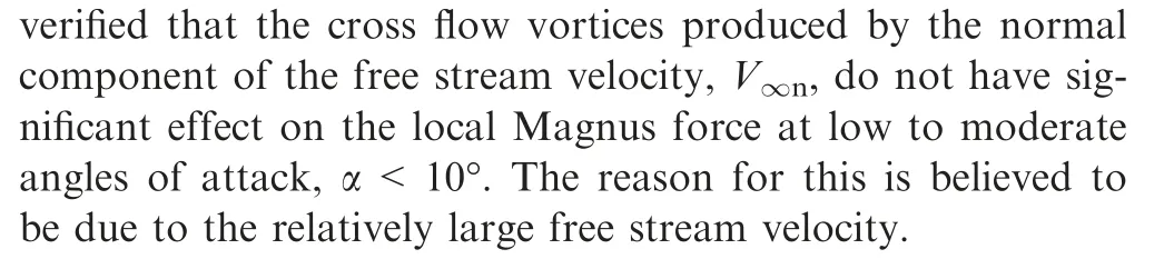
- Strong interactions of incident shock wave with boundary layer along compression corner