Analysis of Unstarted Hypersonic Flow Unsteadiness Based on Schlieren Image Processing

WANG Chengpeng，WANG Wenshuo，XUE Longsheng，XU Pei，YANG Jinfu

College of Aerospace Engineering，Nanjing University of Aeronautics & Astronautics，Nanjing 210016，P.R.China

（Received 5 September 2018；revised 11 February 2019；accepted 2 July 2019）

Abstract: The unstarted flow field in a hypersonic inlet model at a design point of Ma 6 is studied experimentally. The time-resolved spatial flow characteristics of the separation shock oscillation，which is induced by the unstarted flow，are analyzed based on a high-speed Schlieren system and an image processing method. The motion of the separation shock detected by the shock-detection algorithm is compared to the results of fast-response wall-pressure measurements，and good agreement is demonstrated by comparing the frequency components in the power spectral density contours between shock oscillation and pressure fluctuation. The hysteresis of the pressure and separation shock during oscillation cycles is observed from the time history of the shock motion，which means that the unsteady flow pattern of the unstarted hypersonic flow can be accurately clarified by time-resolved Schlieren image processing.These results convincingly demonstrate that the shock - detection technique is successfully applied to an unstarted hypersonic flow case.

Key words: shock-detection system; hypersonic inlet flow; unstarted flow

0 Introduction

Supersonic combustion ramjet（scramjet）propulsion systems have been studied extensively over the past several decades for future air-breathing vehicles［1-3］. The hypersonic inlet，which provides a steady stream compressed air to the combustor，is an important aerodynamic component in scramjet engines. However，the unstart phenomenon of the hypersonic inlet is harmful to the engine and may lead to unsteady and higher aerodynamic and thermal loads on a vehicle’s structure.Several flight tests fail due to unstarted flow of hypersonic inlets，such as the second flight test of the X -51 of the USA. Many review articles have been published on the topic of "the hypersonic inlet unstart"，with different oscillatory flows in different works［4-6］. Despite numerous studies ， the"unstart phenomenon" remains a critical issue in the design of air - breathing vehicles ，and the detailed mechanism of the flow unsteadiness remains unclear.

Fig.1 Flow pattern of hypersonic inlet for the unstart condition

When a hypersonic inlet is operating under the unstart condition，the internal flow in the scramjet engine will change the flow capturing characteristics of the inlet，and the separation shock in the external - compression flow field will oscillate（Fig. 1） around the inlet cowl［7］. The unstart induces severe flow fluctuations，and the transient flow structures that characterize the process of unstart are shock oscillations and wall pressure fluctuations. As a result，a hypersonic inlet unstart is accompanied by induced separation shock （Fig. 1），with airflow spillage above the cowl. The Schlieren technique is particularly suitable for capturing the density jump across the separation shock.Therefore， the unstart detection technique based on high-speed Schlieren images of separation shock is important to characterize the unsteadiness. This diagnostic method shows direct spatial observations of separation shock location. To further characterize the unstarted flow unsteadiness，it is necessary to develop the postprocessing methods that track unsteady separation shock motion in time-resolved high-speed Schlieren images.

Most experimental studies on hypersonic unstarted flow are conducted mainly from two aspects：shock structures analysis by Schlieren technique and data time history/frequency analysis by dynamic wall pressure［8-12］. However， for a long time，Schlieren images have only been used to depict qualitatively typical flow patterns of the unstart process，and the evolution over time of the shock motion has not been taken into account. Few statistical data of separation shock motion induced by unstart in Schlieren image are obtained to analyze the shock unsteadiness accompanied by the unstarted flow. However，based on the statistical analysis of the separation shock oscillation，many novel flow mechanisms of hypersonic inlet unstart would be found. To fill the gap，a particular shock -detection technique and time-frequency method should be developed.

In the present paper， we shall describe the Schlieren image-processing algorithm and shock-detection schemes in detail and then use those tools to exhibit the unsteady shock signal recorded in Schlieren images. Indeed，time - frequency analysis and shock - detection algorithms （which are commonly used in other domains but are almost unusual in the field of unstarted hypersonic inlet aerodynamics）could，in our opinion，be useful for many readers in their analytical works on unstarted hypersonic inlet flow.

1 Experimental Apparatus and Test Model

1. 1 Wind tunnel

The experiments are conducted in the Hypersonic wind tunnel of Nanjing University of Aeronautics and Astronautics（NHW，Fig.2［13-14］）at a nominal free stream Mach number of 6. The wind tunnel runs in a "blow-down-to-vacuum" mode，and the air is supplied by storage tanks with a volume of 32 m3and a pressure of 23 MPa. The converging-diverging nozzle （exit diameter of 500 mm）mounted in the test section is interchangeable and provides nominal free stream Mach numbers from 4.0 to 8.0. The wind tunnel’s run time，which depends on Mach number，is 7—10 s. Two glass windows（diameters of 300 mm）are embedded in two sides of the test section walls for optical access. The air would be inhaled into a vacuum ball（volume of 650 m3）in the downstream of the test section and wind tunnel diffuser. The experiments could be carried out under conditions of 0.04—1.0 MPa total pressure，288—685 K plenum temperature and 6.47×105—2.24×107m-1unit Reynolds number.

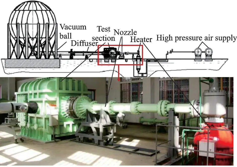
Fig.2 Hypersonic wind tunnel (NHW)

1. 2 Experimental measurements

Fig. 3 shows a schematic of the measurement system setup. Schlieren flow visualization systems are used to obtain the flow characteristics. Each Schlieren system contains light sources，optical devices and a camera. Halogen lamps are used as Schlieren system light sources. A NAC（NAC Image Technology）hotshot high speed camera operated at a frame rate of 5 kHz and a resolution of 600 pixel×438 pixel（1/20 000 s exposure time）is used in the tests.

Fig.3 Schlieren and data acquisition system

The pressure measurement system consists of 16 Kulite XTEL - 190 M fast - response transducers and data acquisition（DAQ）cards（National instruments PXIe 6358）. The 16 transducers are mounted along the central line of the lower wall（Fig.4，T1-T16） from downstream to upstream. In the current tests，the signals of the 16 transducers are acquired at a rate of 10 kHz by the data acquisition cards with a 10 s sampling time，which covers the entire run time of the wind tunnel.

Fig.4 Test model in the wind tunnel

To keep the Schlieren flow visualization synchronized with the pressure signals，a synchronizer is used to trigger the camera and the DAQ pressure acquisition system simultaneously，and the motor is triggered after a delay of 5.6 s.

1. 3 Test model

The test model is a three - dimensional hypersonic inlet（Fig. 5）with the length of 980 mm and has a rectangular exit that is 40 mm in height and 44 mm in width. The inlet’s unstart state is generated by a throttling device with a plug（half-apex angle of 20°）driven by a stepper motor（Fig.5）.

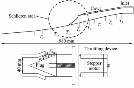
Fig.5 Transducer installation locations and throttling device

A non-dimensional variable Δ is defined to measure the effect of throttling，which can be illustrated as h0= x0⋅sin20° (3)where Atxrepresents the area size that flow can cross the outlet effectively，and A0is the total area of the outlet. The plug driven by a stepper motor that can move 0.01 mm per step ensures an accurate control system.

In the current experiment，the inlet is designed at Ma 6 based on a combination flow field. According to the study conducted by You et al［15］，the basic flow field named ICFC（internal conical flow C），combination of ICFA（internal conical flow A）and Busemann flow［16］，presents better compression performance with limited inlet length. The streamline tracing method［17］is used to shape the inlet walls，and a “V” cowl shape is formed in the roof. As shown in Fig. 6，the ICFA flow section with an edge wedge angle of 6oprovides leading edge shock 1 （shock angle β=13.98o），while the Busemann flow section generates the isentropic compression shocks 2（the shock in the Fig.6 side view is on the symmetry plane of the inlet）. Both the designed leading edge and the separatrix between ICFA and Busemann flow field are curved，but to match the vehicle body design，the curved leading edge is replaced by a straight edge in the actual test model.The contraction ratio of this model is 5.095，and the internal section is 2.171.

Fig.6 Hypersonic inlet in the current test

2 Schlieren Image Analysis and Quantization Method

Due to the restricted area size of the Schlieren window and the opaque side panel， the current study mainly focuses on external flow field. To obtain the motion features of the unstarted separation shock，a quantization method is presented in this paper. It is necessary to introduce this method in detail before acquiring the flow characteristics of the separation shock motion.

The high speed camera used in the test can operate during a usable run time of 6 s at a frame rate of 5 kHz（600 pixel×438 pixel），and 30 000 Schlieren images could be taken in one case. Therefore，the dynamic flow structures can be recorded by image gray scale，and the quantization method is proposed based on the gray level detection. The key steps of the method include state judgment of the flow（start or unstart），separation boundary localization，accuracy judgment and output of the variables（Fig.7）.

Fig.7 Process of the quantization method

2. 1 State judgment

The amount of data from all of the Schlieren images is huge，and the costs in computing resources and time will be too great if every image is employed in the separation boundary localization. Actually，the flow field wherein separation shock does not appear does not need to be calculated. Therefore，the state judgment step is important to the quantization method.

The picture is treated as a gray level matrix G，G0is defined to represent the started flow field（Fig. 8（a）），and Gxrepresents an arbitrary flow field. Here G，G0and Gxare all M×N matrices（M×N：width × height，pixel）.

The matrix Gdxis defined to measure the difference between G0and Gx，which is

Fig.8 Typical flow structures in Schlieren images

where i=1，2，…，M，j=1，2，…，N，which is the same as in the following Eqs.（4，5，7，8）. In fact，even in the started flow，two pictures cannot be identical，which is related to the noise level caused by the wind tunnel and camera. Consequently，finding one image that represents the relatively steady initial started flow is difficult. In the current study ，filtering methods such as median filtering and average filtering have been tested to weaken the influence of noise，but the results are not as expected. In this quantization method，n pictures of started flow are chosen for the relatively steady started flow calculation，and G0can be obtained as

The value of e is defined to measure the noise level of the started flow field，which is

where Gdσxis the variance level，and Gˉdxis the average level of the n pictures. Therefore，e is determined by the average and variance of the noise. A typical vertical line l0located in the intersection between the side and bottom walls is chosen to judge the flow field state. As shown in Fig.8（b），it can be observed from the unstarted flow that the massive separation region traverses l0. yl0xrepresents the gray level difference vector of l0in Gdx，and the value ηxis defined to measure the number of points that exceed the noise level，which is

where ηmaxis defined to measure the state judgment level，and the value is the maximum of ηxamong the n pictures of started flow. Therefore，under the actual free stream flow conditions

It should be noted that the started flow here is the state of instantaneous start and just represents that the separation shock does not appear. Consequently，whether it is the start of an arbitrary Schlieren image can be judged by one value of ηx.

2. 2 Separation boundary localization

When a separation shock appears，its boundary is located in the positive value position of Gdx. To save computational resources，the picture is split by l0，and only the left part is calculated. The ym，Nrepresents one of the vectors in Gdx，where 0 ＜m ≤ml，m is the x coordinate，and mlis the position of l0. hmis the highest y coordinate in ym，Nthat exceeds the noise level.

where ε is the relaxation factor of accuracy，which will be discussed in the next step. Therefore，hmis the separation shock boundary height. The function y = fw( x ) is defined to describe the central line of the bottom wall，and this function is a given condition. m and hmmust satisfy the inequality hm＞fw( m )，and therefore，some of the upstream points should be dropped when the separation point is in the Schlieren image region. m0is defined to represent the lower limit of m，which is

where mmin= min { m | hm＞fw( m ),0 ＜m ≤ml}；ξ is a factor used to control the dropping level and is related to the noise，contrast ratio and window size.In current testing，according to practice and experience，ξ should be set to 0.2. As shown in Fig.9，the separation shock boundary is clearly presented by ym，N.

Fig.9 Boundary line of the separation shock located by the quantization method

Then，the function of separation shock y = k ⋅x + b can be calculated by the least squares method，which is

2. 3 Accuracy judgment

It is obvious that the localization points should present strong linearity and relevance，whereas the correlation coefficient will decrease if there were too many error points. Therefore，the correlation coefficient r is chosen to judge the accuracy. r is calculated by

z is set to 0.1 in this test，and the next step will be taken while r＞r0. A program based on C++code is run to calculate the separation shock from all the pictures. For the accuracy detection，a function to dye the boundary of separation shock is added to the code. By running the program，the separation shock boundary is marked with red lines，and endpoints are marked with square symbols autonomously，so that the deviation of localization can be observed intuitively. Fig.10 shows the contrast between the original and calculated pictures of shock oscillation during one cycle，whose results prove the accuracy and efficiency of this program code.

Fig.10 Localization and dyeing results of separation shock after program running

2. 4 Variables output

For the detailed description of separation shock，four parameters are adopted in the present study（Fig.11）：The displacement of the separation point x，the velocity of the moving separation point v，the angle of the separation shock β and the height of the separation shock boundary in the cross area between the bottom and side wall h.

The four variables can be calculated by

Fig.11 Descriptive parameters of separation shock

It should be noted that if the separation point is outside the picture（Fig. 12），the point will not be marked but still can be calculated.

Fig.12 Calculation of the separation point

3 Results and Discussion

The free stream flow conditions for the current experiment are listed in Table 1.

Table 1 Free stream flow conditions

The motion of the separation shock is described by the quantization method mentioned above，and the data characteristics of the time history are collected，including x，v，β and h. The separation point position x reflects the size of the separation region’s area. v is the velocity of the separation motion. β represents the strength of the separation shock，and h represents the amplitude of the shock oscillation.

During this test，it is found that the occurrence of separation shock oscillation in the cowl area presents various characteristics depending on Δ. To obtain the separation shock at different Δ completely，Δ is set to 0（started flow of inlet）initially when the internal and external flow field of the inlet is established，and the plug then begins to move upstream at a speed of 10 mm/s. Fig.13 shows the time histories of the four variables，in which the leading edge is defined as x = 0 and the free stream direction is defined as positive. And the dynamic wall pressure of the T11signal is also shown，in which T11is located at the foot of the separation shock and its position is shown in Fig.4. In this case，as seen，Δ increases linearly during the test time，while x，v，β，h and pressure of the T11signal change respectively and simultaneously.

Fig.13 Time history of the shock motion parameters and dynamic pressure of the T11 signal

Fig. 14 shows the wavelet transform time - frequency analysis results for the five variables. It is obvious that all of them have a clear basic frequency that keeps increasing from 50 Hz to 120 Hz and several harmonic - frequency components. The frequency regions are formed at t=2.15 s when the shock oscillation occurs. There is a sustained growth during t=2.15—3.86 s，whereas the frequency regions remain relatively stable after that. The typical time segments will be analyzed in detail. Both the data of the unstarted separation shock in the Schlieren image（Figs.14（b-e））and the wall-pressure（Fig.14（a））yield the same change in the dominant frequency，which demonstrate that the shock oscillation and the pressure fluctuation are highly correlated.These results demonstrate the validity and rationality of the Schlieren image-processing method.

Fig.14 Power spectral density contours

Stage 1t=0—2.15 s with Δ＜35.83%. In this stage，a shock train is produced in the isolator with growing back pressure by throttling. Fig. 15 shows the pressure time history of four typical survey points. As seen，T1first senses the back pressure，and the others lag behind in turn when the shock train moves upstream. The pressure fluctuation occurs at t=2.15 s. The PSD of the T1signal is shown in Fig.16，and it demonstrates that the basic frequency is not distinct before t=2.15 s. In the present work，separation shock in the cowl area is mainly focused，and therefore，it is regarded as one stage before separation shock oscillation occurs，which is the stage of start.

Fig.15 Pressure time history at typical survey points

Fig.16 Power spectral density of T1

Fig.17 Partial time history and Schlieren images

Stage 2t=2.15 s—3.86 s with Δ=35.83%—64.33%. A typical time segment t=2—2.5 s is show in Fig.17. In this period，the flow field in the cowl area begins to show the throttling effect of the plug while the inlet is in its early stage of unstart with small amplitude and long cycle of wall pressure and separation shock. The first cycle appears from t=2.151—2.213 s with Δ=35.85%—36.88%. This throttling level is the critical point between start and unstart flow of the inlet. As seen from the Schlieren pictures（Fig.17），the separation shock is shaped at t=2.154 2 s，and the separation bubble propagates rapidly，with point A continuing to move forward.The separation bubble stops propagating at approximately t=2.156 0 s，and the separation shock remains temporarily stable with h≈83 mm and β≈12°. At approximately t=2.158 2 s，the separation bubble begins to move backwards，while the separation shock does not change immediately until it moves back completely after t=2.159 s，when the separation shock disappears. This result demonstrates that the motion of the separation shock moving forward is not the same as when it moves backward. When the separation bubble moves upstream，the separation shock shows a strong following，but when moving downstream，the following is not apparent. Therefore，in one oscillation cycle，the motion of the separation shock moving downstream a has a hysteresis.

Fig. 18 shows the hysteresis of T11wall pressure and variables of separation shock. It is obvious that during one oscillation cycle，the pressure and velocity of the separation point present strong hysteresis，whereas the angle and amplitude of the separation shock are not obvious. It demonstrates that there can be different speeds at which a separation bubble propagates and different wall pressures in the same position as the separation point moves upward and downward.

Fig.18 Hysteresis of pressure and separation shock during the first cycle

Fig.19 Partial time history and Schlieren images

Stage 3t=3.86—6 s with Δ ＞64.33%. A typical time segment of t=5.6—5.7 s is shown in Fig. 19. Schlieren images obtained during the t=5.634—5.641 s cycle are presented. As seen，at t=5.637 6 s，the separation shock reaches the highest position，which is higher than that in stage 2，and the separation point has reached the leading edge in every cycle. It is similar to stage 2 when the separation point continues to move upstream but is different in that the separation shock in the cowl area is almost straight when it reaches the highest position.In this stage，the basic frequencies of the variables are stable （Fig. 14） and cycles demonstrate little change in length，but some variables，such as h and P11，grow in amplitude with the increasing back pressure. The second harmonic frequencies of P11，v and β are stronger，while those for x and h are weaker.

In this flow structure，the separation point can reach the leading edge，and the separation bubble spreads to the entire bottom wall. Then the leading edge shock disappears and is replaced by a separation shock. Fig.20 shows the pressure time history of four typical survey points. The T13—T16signal pressures show strong correlation，and their fluctuation amplitudes increase obviously in comparison with stage 2.

Fig.20 Pressure time history of typical survey points

4 Conclusions

In the present study，a hypersonic inlet model is tested in a Ma 6 free stream in a hypersonic wind tunnel. The inlet unstart phenomenon in external flow is the primary focus. During the test，the unstarted flow is generated by a continuously increasing throttling device at the exit of the isolator. A high speed Schlieren system and fast response pressure transducers are used to obtain the dynamic flow structure. From the analysis of Schlieren images and dynamic pressure， some novel methods are proposed，and the following conclusions are obtained.

The method of image quantization of Schlieren photographs is practical，and a dynamic flow structure can be shown in detail by catching the features of separation shock in the pictures. More information about shock than wall pressure can be obtained.By using this method，the unsteady flow pattern of the unstarted hypersonic flow is clarified based on time-resolved Schlieren images of separation shock.In the present experiment，the basic frequencies of shock oscillations and pressure fluctuations in unstarted flow range from 50 Hz to 110 Hz，and the second harmonic frequencies are 100 Hz to 220 Hz.The frequency components have an obvious increase with the continuously increasing throttling，but they will remain relatively stable when the separation shock amplitude reaches the position of the leading edge shock and intersects each other upstream.