Global and Bifurcation Analysis of an HIV Pathogenesis Model with Saturated Reverse Function

Liu Yong-qi and Meng Xiao-ying

(1. College of Applied Mathematics, Beijing Normal University, Zhuhai, Guangdong, 519087)

(2. School of Statistics and Mathematics, Zhongnan University of Economics and Law,Wuhan, 430073)

Communicated by Shi Shao-yun

Abstract: In this paper, an HIV dynamics model with the proliferation of CD4 T cells is proposed. The authors consider nonnegativity, boundedness, global asymptotic stability of the solutions and bifurcation properties of the steady states. It is proved that the virus is cleared from the host under some conditions if the basic reproduction number R0 is less than unity. Meanwhile, the model exhibits the phenomenon of backward bifurcation. We also obtain one equilibrium is semi-stable by using center manifold theory. It is proved that the endemic equilibrium is globally asymptotically stable under some conditions if R0 is greater than unity. It also is proved that the model undergoes Hopf bifurcation from the endemic equilibrium under some conditions. It is novelty that the model exhibits two famous bifurcations,backward bifurcation and Hopf bifurcation. The model is extended to incorporate the specific Cytotoxic T Lymphocytes (CTLs) immune response. Stabilities of equilibria and Hopf bifurcation are considered accordingly. In addition, some numerical simulations for justifying the theoretical analysis results are also given in paper.

Key words: HIV model; global asymptotical stability; center manifold theory; Hopf bifurcation; backward bifurcation

1 Introduction

Human Immunodeficiency Virus (HIV), which destroys CD4 T cells and decreases the resistance of the immune system. The count of CD4 T cells is a primary indicator used to measure progression of HIV infection. In a normal healthy individual’s blood, the level of CD4 T cells is between 800 and 1200 mm−3(see [1]–[3]). When CD4 T cells count of one patient reaches 200 mm−3or below, the person is called AIDS patient. The amount of virus rises dramatically after primary infection and falls to a lower level after a few weeks to months. At first, it is estimated that as many as 1010virions are produced and destroyed in an infected individual each day. The amount of virus rises again after ten years or so (see [1]).By utilizing mathematical models, we can better understand HIV dynamics, disease progress and interaction of HIV and the immune system. Many ordinary differential equations for HIV infection pathogenesis have been proposed and investigated by bio-mathematicians (see[1] and [3]–[5]). The basic mathematical model which describes HIV infection dynamics has been studied in [1] and [4]. Global stabilities have been established by using Lyapunov functions. Many papers consider the proliferation of the CD4 cells (see [3] and [6]). Motivated by the above works, we propose one HIV model which is described by the following system of differential equations

State variables T(t), T∗(t) and v(t) represent the concentration of uninfected CD4 T cells,infected CD4 T cells, and the HIV particles in the blood, respectively. The human body produces CD4 T cells at a constant rate s. The parameters δ, a and c denote the death rate of uninfected CD4 T cells, infected CD4 T cells and the virus particles, respectively. Here we use bilinear incident rate βT(t)v(t) to describe the infection incident rate. The termdenotes saturated reverse function response, the proliferation of CD4 T cells,where r is the maximal proliferation rate, k is half-saturation constant of the proliferation process and can be considered as michaelis-menten constant. Free HIV are produced from actively infected cells at rate bT∗(t) and are removed at rate cv(t).

The main purpose of this paper is to analyse global properties for the system (1.1)–(1.3)and explore the impact of saturated reverse function response on the dynamical behavior of the system. We begin model analysis with proving the positivity and boundedness of the solutions of the system. We prove that system (1.1)–(1.3) exhibits the backward bifurcation and Hopf bifurcation under some conditions. We prove that the endemic equilibrium is globally asymptotically stable under some conditions by using the geometric approach,developed by Li and Muldowney (see [2], [7]–[8]). We also research the effect of CTLs on HIV infection and give the conditions of Hopf bifurcation.

This paper is ordered as follows: equilibria, properties analysis are studied when R0< 1 in Section 2. In Section 3, the global asymptotical stability of the endemic equilibrium and Hopf bifurcation are investigated when R0> 1. In Section 4, we consider the extended system and explore its stability and bifurcation. Section 5 gives numerical results for the system. Section 6 is conclusions. Section 7 is Appendix.

2 Equilibria and Stability when R0 < 1

Before HIV infection invades the host, we have T∗= v = 0. It can be shown that CD4 T cells converge to the value T =. We note that the basic reproduction number R0for the system is given by

If R0< 1, this means that an infected cell will on average produce less than one infected cell. The HIV infection cells are cleared from the CD4 T cells population. If R0> 1, this means that an infected cell will on average produce more than one newly infected cell in the host. The HIV infection will persist in the host. In classic epidemic theory, the basic reproduction number largely determines whether infection will be sustaining in a certain degree. We easily get the following results by letting the right sides of system (1.1)–(1.3) be zero.

Proposition 2.1For the system(1.1)–(1.3),

(1)the system always exists one nonnegative equilibrium,which representsthe state that the virus are absent;

(2)the system has one positive equilibriumifR0< 1andr = βk + δ(1 −

(3)the system has two positive equilibriaifR0≤1and

(4)the system has only one positive equilibriumP4(T4,, v4)ifR0> 1;

(5)otherwise,the system has no positive equilibrium,where

Proposition 2.2All the solutions of the system(1.1)–(1.3)with positive initial conditionsT(0) > 0, T∗(0) > 0, v(0) > 0remain positive for allt ≥0.

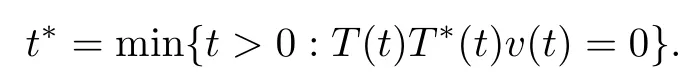
Proof.Assume that there exists t > 0 at which T(t), T∗(t) or v(t) is equal to 0. Denote

If T(t∗) = 0, it follows that

However, from T(0) > 0 and T(t∗) = 0, we can obtain

That is a contradiction. Thus T(t) > 0 for all t ≥0. If T∗(t∗) = 0, it follows that T(t∗) > 0,v(t∗) ≥0 when t ∈[0, t∗]. Then

But we know that the set

is an invariant set with respect to system (1.1)–(1.3). So we get v(t∗) > 0. Therefore,

However, from T∗(0) > 0 and T∗(t∗) = 0, we can obtain

That is a contradiction. Thus T∗(t) > 0 for all t ≥0. In a similar way, we can obtain v(t) > 0 for all t ≥0. Solutions remain positive for positive initial conditions. This completes the proof.

Proposition 2.3Whenβk + δ ≥r,for any positive solution of system(1.1)–(1.3)and sufficiently larget,there existsM > 0such thatT(t) < M, T∗(t) < Mandv(t) < M.

Proof.We obtain

from (1.1) when

if r − βk ≤0, it is easy to get that T(t), T∗(t), v(t) are bounded. So we get

So there exists M1such that T ≤M1. Furthermore, we get

Then there exists M2> 0 such that T∗≤M2. Similarly, there exists M3> 0 such that v ≤M3. Therefore, we can obtain boundedness of T(t), T∗(t), and v(t) when v > v0.

If v ≤v0, we obtain

It follows from (2.1) that T(t) is bounded. Similarly, T∗(t) and v(t) are also bounded as well. So we show that all solutions of system (1.1)–(1.3) are uniformly bounded, say by M.This completes the proof.

Define the region

where R3+denotes the non-negative cone. Obviously, solutions of system (1.1)–(1.3) remain non-negative for non-negative initial conditions. So P is a positively invariant set with respect to system (1.1)–(1.3). In the following, we investigate dynamic behavior in P.

Theorem 2.1For system(1.1)–(1.3),whenβk + δ ≥r,

(1)the disease-free equilibriumP0is local asymptotically stable inPifR0< 1and is unstable ifR0> 1;

(2)ifP2andP3both exist, P3is locally asymptotically stable andP2is unstable;

(3)ifP1exists,it is semi-stable.

Proof.The Jacobian matrix of system (1.1)–(1.3) at P0is computed to be as

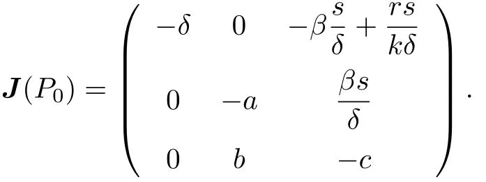
It is easy to see that all roots of the characteristic equation at P0have negative real parts if R0< 1, thus P0is locally asymptotically stable. The characteristic equation about P0has at least one positive root if R0> 1, therefore, P0is unstable.

The Jacobian matrix corresponding to Pi(i = 1, 2, 3) is given by

The characteristic equation corresponding to Pi(i = 1, 2, 3) is given by

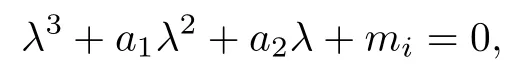
where

Denote

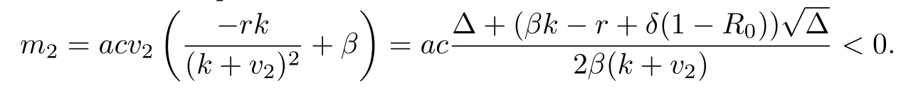
We calculate m2and acquire

We also compute m3and acquire

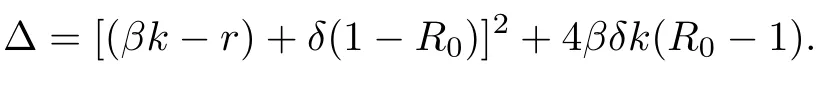
We also have

Since βk + δ ≥r, we obtain

Therefore, a1a2−m3> 0 and P3is locally asymptotically stable.

In the following, we discuss the local asymptotical stability of P1. Since the characteristic equation around P1has two negative real parts roots and one zero root, we use the method of center manifold theory (see [9]–[10]).

Denote

Therefore, system (1.1)–(1.3) changes into

Under non-singularity transformation

the system (2.3)–(2.5) becomes into the following form

For system (2.6)–(2.8), we can get a local center manifold that has the form as follows:Then we let

By simply computing, we obtain the solutions on the center manifold satisfy

We can see that the disease will not die out under some conditions even R0< 1. Whether we can eradicate the disease or not is relate to the initiate states. We can see a stable endemic equilibrium coexists with a stable disease-free equilibrium when the associated reproduction number is less than unity. That is to say, the system can exhibit the phenomenon of backward bifurcation.

Theorem 2.2IfR0≤1andβk ≥rhold,the disease-free equilibriumP0is globally asymptotically stable inP.

Proof.When βk ≥r, there is no other steady state except for P0if R0≤1 from Proposition 2.1. We define a Lyapunov function

Then the derivative of L along the solution of system (1.1)–(1.3) is

3 Global Stability and Hopf Bifurcation when R0 > 1

Theorem 3.1Suppose thatR0> 1andβk +δ ≥r,the endemic equilibriumP4is locally asymptotically stable.

Proof.The characteristic equation corresponding to P4is given by

where

It can be seen easily that

Next we discuss the global asymptotical stability of the endemic equilibrium P4by using the geometric approach based on the second additive compound matrix (see [2], [7]–[8]).

Definition 3.1[7],[11]System(1.1)–(1.3)is said to be uniformly persistent if there exists a constantm > 0such that each positive solution(T(t), T∗(t), v(t))with initial conditions in the interior ofPsatisfies

Proposition 3.1(1.1)–(1.3)is uniformly persistent in the interior ofPifR0> 1.

Proof.When R0> 1, we see that P0is unstable. Solution which close to P0will leave its neighborhood except for solutions on the positively invariant T-axis. The interested reader can see [2], [7], [12]–[13].

Theorem 3.2The endemic equilibriumP4of(1.1)–(1.3)is globally asymptotically stable inPifδ > randR0> 1.

Proof.We use Lemma 7.1 in Appendix to prove the global asymptotical stability of endemic equilibrium. From above discussion, we know that interior of P is simply connected and P4is unique equilibrium in the interior of P. Both (H1) and (H2) in Appendix are satisfied. The uniform persistence of system when R0> 1, together with the boundedness of solutions, implies the existence a compact absorbing set E ⊂P (see [2], [7]). This verifies the assumption (H3) in Appendix. P4is locally asymptotically stable when δ > r from Theorem 3.1. The Jacobian matrix J of system (1.1)–(1.3) is given as

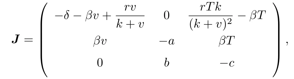
and its second compound matrix J[2]

Denote the function Q = Q(T, T∗, v) =, then

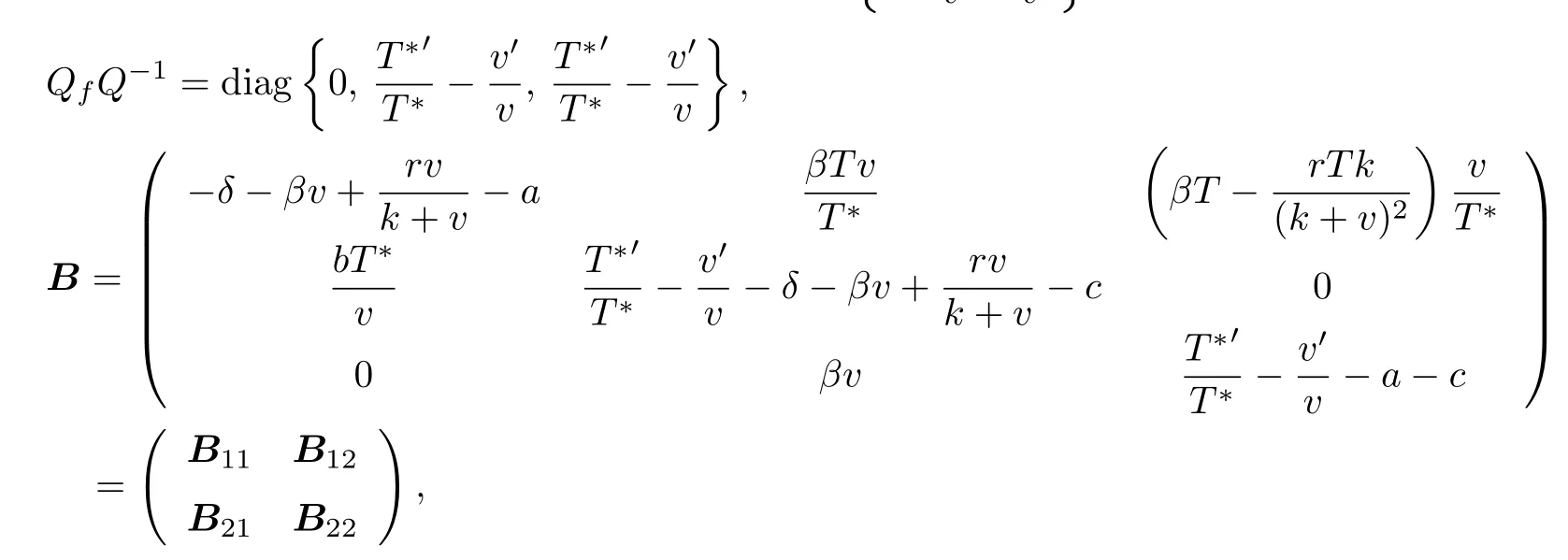
where

Let (u, v, w) denote the vectors in R3, choose a norm in R3as

and let µ be the correspondingmeasure (see [2], [12]). Then we have

where g1= µ(B11) + ∥B12∥, g2= µ(B22) + ∥B21∥, and where ∥B12∥, ∥B21∥are matrix norm with respect to l1vector norm. Then we obtain

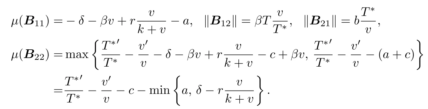
Because of δ > r, we obtain that

From system (1.1)–(1.3), we have

Hence,

Therefore we get

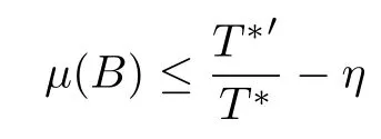
for sufficiently large t with η = min{a, δ −r}.

Now, let (T(t), T∗(t), v(t)) be any solution starting in the compact absorbing set E ⊂P andbe sufficiently large such that (T(t), T∗(t), v(t)) ∈E for all t >. For t >, we have

This completes the proof.

Meanwhile, we obtain that

maybe less than 0 by numerical simulations if βk + δ < r. Thus the Routh-Hurwitz criteria may not always be satisfied. So it is possible to occur Hopf bifurcation around positive interior equilibrium P4. That is, a branch of periodic solutions splits off from an equilibrium when some parameters change. Here we have taken r as a bifurcation parameter.

Theorem 3.3IfR0> 1,then system(1.1)–(1.3)aroundP4undergoes a simple Hopf bifurcation whenrpasses through one certain valuer0,which satisfiesa1(r)a2(r) = m4(r).

Proof.Denote

Now we can obtain r = r0from ψ(r) = 0 and we have a1(r) > 0, a2(r) > 0, and m4(r) > 0.(3.1) is given by

It is easy to see that (3.2) have a pair of purely imaginary eigenvalues and a strictly negative real eigenvalue. For r in a neighbourhood of r0, the characteristic equation (3.1)have a pair of complex eigenvalues λ(r) = p1(r) + ip2(r), ¯λ(r) = p1(r) −ip2(r), which are purely imaginary eigenvalues at r = r0. Substituting λ(r) = p1(r) + ip2(r) into (3.1)and calculating the derivative, we obtain that the transversality condition is completely equivalent to ψ′(r0)≠ 0 (see [9]). That is,

By calculating we get

where

Therefore, we derive that the transversality condition (H5) in Appendix holds. The conditions for Hopf bifurcation theorem are verified. This completes the proof.

4 The Extended Model

CTLs response is one major branch of the immune system to fight virus infections and it has been proved to have the potential to suppress HIV load. CTLs kill infected cells and enhance the immune response against HIV to get achieve long-term immunological control of the virus in the absence of continuous therapy (see [14]–[15]). An effective, sustained CTLs response can be established if virus load is contained at low levels. R denote the concentration of CTLs. m1T∗R is the clearance rate of infected cells by CTLs, and m2T∗R is the production rate of CTLs. Meanwhile, we use m2T∗to be production rate. d is the natural death term of R. The expanded model is

We derive

which represents the basic reproduction number of system (4.1)–(4.4). We have the following results:

Proposition 4.1For system(4.1)–(4.4),

(1)the system always exists one nonnegative equilibrium,which repre-sents the state that the virus is absent;

(2)the system has another non-negative equilibrium(T1, T∗1, v1, 0)ifR0< 1, R1< 1,and

(3)the system has two non-negative equilibrium(T2, T∗2, v2, 0),(T3, T∗3, v3, 0)ifR0≤1, R1< 1,andr > βk + δ(1 −R0)+

(4)the system has only one non-negative equilibrium(T4, T∗4, v4, 0)ifR0> 1andR1< 1;

(5)the system has only one positive equilibrium(T5, T∗5, v5, R5)ifR1> 1;

(6)otherwise,the system has no positive equilibrium,whereTi, T∗i, vi(i = 1, 2, 3, 4)are the same as those in Section2,

From the Jacobian matrix at, we get Piandhave the same local asymptotical stability if<(i = 1, 2, 3, 4). If>,(i = 1, 2, 3, 4) is always unstable. We obtain ¯P0is locally asymptotically stable whenever R0< 1. The equilibrium P5contains CTLs immune response. When R0< 1 and (βk −r)cm2+ βbd ≥0, P5does not appear.When R0> 1 and (βk −r)cm2+ βbd < 0, P5exists. The Jacobian matrix at P5is

with the characteristic equation

where

By the Routh-Hurwitz conditions, all eigenvalues of (4.5) have negative real parts if and only if

Theorem 4.1IfR1> 1andβ ≥,then system(4.1)–(4.4)aroundundergoesan Hopf bifurcation whenapasses througha0.

Proof.Let φ(a) = q1(a)q2(a)q3(a) −(a) −(a)q4(a) be differentiable function with respect to a. Suppose β ≥, the conditions of qi> 0 (i = 1, 2, 3, 4) are established.By solving the equation ψ(a) = 0, we can obtain that there exists a = a0such that ψ(a0) = 0.At a = a0, the characteristic equation (4.5) becomes

It is clear that the condition (H4) in Appendix holds. We also obtain

Thus the condition (H5) in Appendix are verified. This completes the proof.

5 Numerical Simulations

In this section, we carry out numerical simulations using Matlab to illustrate theoretical results. Our parameters mainly come from [3] and [6] and our adjustment. Fig. 5.1 shows the simulation of the system (1.1)–(1.3) with the parameter values s = 0.46, δ = 0.003,β = 1 × 10−8, r = 0.002, a = 0.06, b = 2600, c = 0.09, k = 9.5, where the initial conditions x0= [1000; 50; 500]. We get R0= 0.7383 < 1. The solution trajectories tend to the stable equilibrium P0. And Fig. 5.2 shows the simulation of the system (1.1)–(1.3) with the parameter values s = 0.46, δ = 0.003, β = 1 × 10−8, r = 0.002, a = 0.06, b = 2600, c = 0.09,k = 9.5, where the initial conditions x0= [500; 100; 500]. we get R0= 0.7383 < 1. The solution trajectories tend to the stable equilibrium P3. We can see that system (1.1)–(1.3)has two locally stable equilibria (P0and P3) under the same parameters when R0< 1. The different initial conditions can lead to disappearance of the HIV infection or persistence.This phenomenon denotes the disease can not be eradicated only if R0< 1.

Fig. 5.1

Fig. 5.2

Fig. 5.3 shows the simulation of the system (1.1)–(1.3) with s = 0.46, δ = 0.003,β = 1 × 10−8, r = 0.02, a = 0.06, b = 2600, c = 0.09, k = 9.5, where the initial conditions x0= [500; 100; 500]. We get R0= 0.7383 < 1. The stable periodic solutions occur. When the maximal proliferation rate r change the value, we find the system (1.1)–(1.3) exhibits periodic solutions though we do not give proof even if R0< 1. The maximal proliferation rate r plays a vital role in describing the behavior of system (1.1)–(1.3).

Fig. 5.3

For the following parameter values: s = 0.46, δ = 0.0002, β = 1 × 10−8, r = 0.0001,a = 0.06, b = 2600, c = 0.09, k = 9.5, where the initial conditions x0= [500; 100; 500].We get R0= 11.07 > 1. the conditions of Theorem 3.2 are satisfied. Then the positive equilibrium P4is globally asymptotically stable (see Fig. 5.4).

Fig. 5.4

Increasing the maximal proliferation rate r = 0.02, we observe that the system enter into an oscillatory steady state from a stable situation. Fig. 5.5 shows that the simulation of system (1.1)–(1.3) with s = 0.46, δ = 0.0002, β = 1 × 10−8, r = 0.02, a = 0.06, b = 2600;c = 0.09, k = 9.5, where the initial conditions x0= [500; 100; 500]. We get R0= 11.07 > 1.The figure exists a stable periodic solution around P4. We derive that the bifurcation parameter r0≈0.009 from the equation a1(r)a2(r) −m4(r) = 0. Theorem 3.3 is verified.

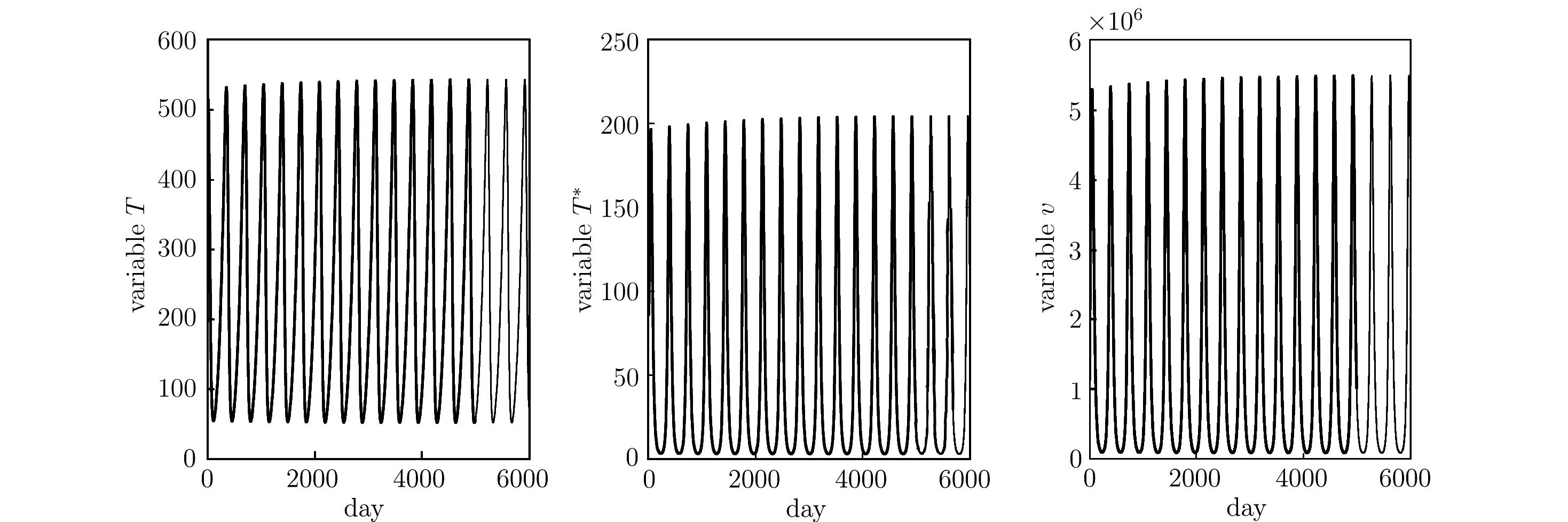
Fig. 5.5

6 Conclusions

In this paper, a deterministic HIV model for the transmission dynamics of nonlinear proliferation is designed and considered. Theoretical results and numerical simulations of the model have been shown. We investigated the qualitative behavior of the model such as positive invariance, boundedness, global stability and bifurcation. The basic reproduction number R0is obtained. It is not sufficient for disease elimination owing to the phenomenon of backward bifurcation. The disease can persist even R0< 1 and also persist when R0> 1.We have shown that there exists a critical value of the proliferation rate r, for which Hopf bifurcation takes place. That is, the asymptotically stable endemic equilibrium loses its stability and periodic oscillation appears. It is shown that system (1.1)–(1.3) also exhibits sustained oscillations from Fig. 5.3. Our system reveals many biology phenomena. The basic model in [4] can not exhibit bifurcation and sustained oscillations. It also is worth mentioning that, sustained oscillations, which can occur for biologically realistic parameter values (see [16]), are significant phenomena for many classes of epidemic models. Equilibria and Hopf bifurcation of the extended model with the CTLs response have been discussed and the conditions have been derived for the stability and Hopf bifurcation.

7 Appendix

We briefly describe below the geometric approach based on the second additive compound matrix, developed by Li and Muldowney (see [2], [7]–[8]). Let an open set D ⊆Rnand the map f : x −→f(x) ∈Rnfor x ∈D. Consider the differential equation

Let x(t, x0) is the solution of (7.1) such that x(0, x0) = x0. We assume that

(H1) D is simply connected,

(H2)is only equilibrium point of (7.1) in D,

(H3) there is a compact absorbing set E ⊂D.

One set E is called absorbing in D for system (7.1) if x(t, E1) ⊂E for each compact set E1⊂E for sufficiently large t. For any square matrix B, themeasure (see [2])with respect to induced matrix norm ∥ · ∥is defined as

We define

The matrix Qfis obtained by replacing each entry qijof Q by its derivative in the direction of f, and J[2]is the second additive compound matrix of the Jacobian matrix J of system(7.1) (see [2]). If M = (mij) is a 3 × 3 matrix, then

In summary, the following result is established:

Lemma 7.1For system(7.1),if assumptions(H1), (H2)and(H3)hold,then the unique equilibriumis globally asymptotically stable inDif there exists a functionQ(x)and ameasureµsuch that< 0.

Hopf bifurcation theorem is stated as follows (see [9], [17] and [18]).

Lemma 7.2Consider system of differential equations with a single parameter

with an equilibrium(x0, µ0),andf ∈C∞.Assume that

(H4)the Jacobian matrixDxfµ0(x0)has a simple pair of pure imaginary eigenvalues and other eigenvalues have negative real parts. Then there exists a smooth curve of equilibria(x(µ), µ)of(7.2)withx(µ0) = x0. The eigenvalues(λ(µ),(µ))ofDxfµ(x)which are pure imaginary atµ = µ0vary smoothly with respect toµ. Moreover,if

(H5)the transversality condition

Then a simple Hopf bifurcation occurs atµ = µ0.