Global Existence and Blow-up for a Two-dimensional Attraction-repulsion Chemotaxis System

Xiao Min and Li Zhong-ping

(College of Mathematic and Information, China West Normal University, Nanchong,Sichuan, 637002)

Communicated by Wang Chun-peng

Abstract: This paper is devoted to dealing with the parabolic-elliptic-elliptic attraction-repulsion chemotaxis system. We aim to understand the competition among the repulsion, the attraction, the nonlinear productions and give conditions of global existence and blow-up for the two-dimensional attraction-repulsion chemotaxis system.Key words: chemotaxis; attraction-repulsion; global boundedness; nonradial solution; blow-up

1 Introduction

Chemotaxis is a phenomenon which describes the movement of cells in response to the concentration gradient of the chemical produced by cells themselves. The famous chemotaxis model was first proposed by Keller and Segel[1]in 1970. The Keller-Segel model can be read as follows:

where u = u(x, t) denotes the density of cells, v = v(x, t) represents the concentration of the chemoattractant. The function f : [0, ∞) −→R is smooth, χ is the parameter referred as chemosensitivity. The system (1.1) with τ = 0 or τ = 1 has been studied extensively in the past four decades. For instance, when D(u) ≡1, τ = 0 andΩ⊂R2is a bounded domain, the solution to (1.1) is global bounded provided that f(u) = µu(1 −u) with µ > 0(see [2]).

In order to better understand the parabolic-elliptic-elliptic attraction-repulsion chemotaxis system, let us mention previous contributions as follows:

When n = 1, the main results in [3] showed that the (1.2) admits a unique global solution. Nagai[4]found that there exists the critical mass mc=which determines the behavior of the solution when n = 2. Precisely, if the initial mass(x)dx ≤mc, the solution of system (1.2) is global and bounded, whereas the finite time blow-up happens when. In addition, the blow-up may occur whenin some specialΩ(see [5]–[8]). When n ≥3, Winker[9]showed that there exists radially symmetric solution blowing up in finite time with proper initial conditions.

In numerous biological processes, general mechanisms in cell include not only attractive but also repulsive signals, which can form various interesting biological patterns (see [10]).Then the model can be expressed as following attraction-repulsion chemotaxis system:

The system (1.3) is proposed by [11] to describe the aggregation of microglia observed in Alzheimer’s disease. Fewer blow-up results are available for system (1.3) than (1.1),because (1.3) relies on Lyapunov function. When n = 1, τ = 1, global existence, non-trivial stationary, asymptotic behavior and pattern formation of solutions to the system (1.3) have been studied in [12]–[13]; when n = 2, τ = 1, if β≠ δ and repulsion prevails over attraction(i.e., ξγ −χα > 0), then the system (1.3) admits a unique global bounded solution (see [14]);in the case τ ≡0, Yuet al.[15]proved that the finite time blow-up for the nonradial solution happens when

when δ ≥ β, or

if δ < β. For more detail results on attraction-repulsion chemotaxis system, we refer the readers to [17]–[20]. Blow-up is an extremely behavior. In order to restrain the behavior,people add the logistic source. More detail results on attraction-repulsion chemotaxis system with the logistic source, the readers can see [21]–[24].

Inspired by above papers, this paper mainly aims to understand the competition among the repulsion, the attraction, the nonlinear productions. Precisely, we consider the global boundedness and the finite time blow-up of solutions to the following parabolic-ellipticelliptic attraction-repulsion chemotaxis system:

where u = u(x, t) denotes the density of cells, v = v(x, t) represents the concentration of the chemoattractant, w = w(x, t) is a secondary chemical signal as a chemorepellent which mediates the cell’s chemotactic response to the chemoattractant v.Ωis a bounded domain in R2with smooth boundary ∂Ω,denotes the derivative with respect to the outer normal.χ, ξ > 0, α, β, γ, δ > 0, q ≥1, r ≥1 and the nonnegative initial data u0(x) ∈C0(). In this model, the behavior of solutions relies on the interaction between the attraction and repulsion, with nonlinear productions.

The main results of this paper read as follows:

Theorem 1.1(i)Ifq < r,then the system(1.4)has a unique nonnegative and globally bounded solution;

(ii)Ifq = randχα − ξγ < 0,then the solution of(1.4)is globally bounded.

Theorem 1.2Let Ω∈R2be a smooth bounded domain andx0∈Ω. Assume thatis small enough. Then if either of the following case holds:

(i) q = r, χα − ξγ > 0,and

(ii) q > r, χαq − ξγr > 0,the solution of(1.4)blows up in finite time.

This paper is structured as follows. In Section 2, we collect some preliminaries which are used later. Section 3 is devoted to proving Theorem 1.1. Finally, we give some blow-up conditions for the system (1.4), and prove Theorem 1.2 in Section 4.

2 Preliminaries

In this section, we collect some classical conclusions as preliminaries. We begin with the local existence of solutions to (1.4).

Lemma 2.1[7],[15],[16]Assume thatu0(x) ∈C0()is nonnegative in Ω. Then there exists a unique triple(u, v, w)of nonnegative functions fromC0(Ω× (0, Tmax)) ∩C2,1(Ω×(0, Tmax))withTmax∈(0, ∞]solving(1.4)in the classical sense. Furthermore,ifTmax< ∞,then

Lemma 2.2[7],[15],[16]Letube the solution of

whereB := {x ∈R2| |x| < R}andf ∈Lp(B), 1 ≤p ≤ ∞. Then

whereG(x, y)is the green function of−∆onBwith homogeneous Dirichlet boundary condition. Besides, G(x, y)satisfies the following properties:

(i) G(x, y) = N(x−y)+K(x, y),whereN(x−y) = −log |x−y|andK ∈C2(B ×B);

(ii) G(x, y) = G(y, x)forx, y ∈;

(iii) |∇xG(x, y)| ≤onB × Bfor someC > 0.

Lemma 2.3[7],[15],[16]Letu ∈C2()satisfy

withf ∈C0(¯Ω), ρ > 0. Then there exist positive constantsCmandCnsuch that

We define the functionϕ ∈C1([0, ∞)) ∩W2,∞((0, ∞))withr2> r1> 0by

where

Lemma 2.4[7],[15],[16]We construct Φ(x) := ϕ(|x|) ∈C1(R2) ∩W2,∞(R2),which satisfies the following

and

Moreover

whereBi:= {x ∈R2| |x| < ri}withR, ri> 0, i = 1, 2, 3, 4.

3 Global Boundedness

Lemma 3.1[22]Let(u, v, w)be a nonnegative local solution to(1.4)ensured by Lemma2.1. Then for anyη > 0, θ > 1,there isc1= c1(η, θ) > 0such that

and

Proof.We integrate the first equation of (1.4) with respect to x ∈Ωand obtain

so

The second equation of (1.4) implies

Multiply the second equation of (1.4) by vθ−1, then integrate overΩand by Young’s inequality, we get

Then we can know that

In view of Ehrling’s lemma, for any η > 0, θ > 1, there exists a c2= c2(η, θ) > 0 such that

with c3= c3(η, θ) > 0. Since 1 ≤q ≤qθ, by the interpolation inequality, the Young’s inequality and (3.3), we have

Similarly, (3.2) can be obtained by the same procedure as above. This completes the proof.

Proof of Theorem 1.1We begin with showing that for any p > 1, there exists a c = c(p) > 0 such that

Multiply the first equation of (1.4) by up−1and then integrate overΩ, we obtain that

By Young’s inequality with (3.2) and η > 0, we have

where c5= c5(p, η) > 0, c6= c6(p, η) > 0. Hence

Case 1. Let q < r, by Young’s inequality, we have

with c7= c7(p) > 0. We know from (3.11) and (3.12) that

where c8= c6+ c7. We let η =, hence

Due to Young’s inequality, there is a c9= c9(p) > 0 such that

From (3.13) and (3.14), we obtain

with c10= c8+ c9. This implies (3.9).

Case 2. If q = r, we know from (3.11) that

If χα − ξγ < 0, taking η => 0, we have that

By Young’s inequality, there exists c11= c11(p) > 0,

We get from (3.15) and (3.16) that

with c12= c6+ c11. This implies (3.9).

Now, we show that

with some C > 0, which concludes Tmax= ∞by Lemma 2.1.

Case 1. Let p0> max{rn, 1}. Applying an elliptic Lpestimate to the third equation in(1.4) we get from (3.9) that

with C0> 0. Then by the Sobolev imbedding theorem with c0> 0, we have that

We get from (3.10) and (3.18) that

Case 2. Let q < r. By Young’s inequality, we have that

Combining (3.19)–(3.21), we have that

and then

For any t ∈(0, Tmax), we have that

and thus (3.17) is obtained.

Let q = r, (3.19) becomes that

By Young’s inequality and χα − ξγ < 0, we know that

From (3.22) and (3.33), we can obtain that

and hence

Obviously,

Thus (3.17) is obtained.

The proof of Theorem 1.1 is completed.

4 Blow-up of Nonradial Solutions

Let (u, v, w) be the local solution of (1.4) ensured by Lemma 2.1. We should show Tmax<∞. It suffices to find a T > 0 such that theΦ-weighted integral of u(x, t) tends to zeros as t →T. Inspired by [7], [15], [16], this is realized by the following propositions.

Proposition 4.1Letq = r, x0∈Ω and0 < r1< r2< dist(x0, ∂Ω),wheredist(x0, ∂Ω)denotes the distance betweenx0and∂Ω. Then there existC1, C2> 0relying onr1, r2,dist(x0, ∂Ω)such that fort ∈(0, Tmax),

where Φ(x) = ϕ(|x|)defined by Lemma2.1.

Proof.We proceed somewhat similarly to [7] and [16]. Without loss of generality, we suppose that x0is the origin. Multiply the first equation of (1.4) byΦ(x) and integrate overΩ. Since the Neumann boundary condition of (1.4),with r2< dist(x0, ∂Ω) by Lemma 2.4, we know that

By ∆Φ ≤4 onΩ(see (2.3) and (2.4) ) andu0(x)dx, one has

Take r3, r4> 0 such that 0 < r2< r3< r4< dist(x0, ∂Ω) and define ζ ∈(R2) with 0 ≤ ζ ≤1 satisfying

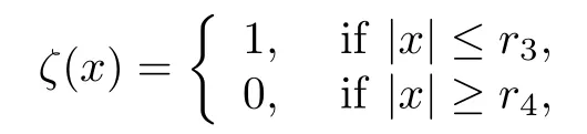
and h(x, t) := ζ(x)v(x, t). By the second equation of (1.4), it is easy that we can verify that h(x, t) satisfies

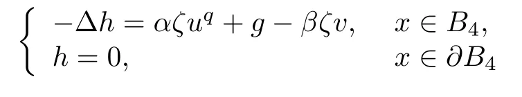
for t ∈(0, Tmax), where g := −2∇ζ · ∇v − ∆ζv. By Lemma 2.2, h(x, t) can be expressed as follows

Since ∇Φ≡0 outside of B2by Lemma 2.4 and h ≡v in B3, we can obtain that

In the following we firstly estimate on I. Since Lemma 2.2(i) with ζ = 1 in B3,

Because of the symmetry property of integrals and ∇Φ≡0 outside B2, we get from the estimate (2.5), (2.6) andΦ≥outside B1that

and

and

So

According to Lemma 2.2(ii), I3can be expressed as follows:

Thus we obtain the estimate

Now, we estimate II. Since g := −2∇ζ · ∇v − △ζv in B3, we obtain by Lemma 2.2(iii)and the H¨older’s inequality that

with C3, C4> 0.

To calculate further, we apply Lemma 2.3 to the third equation of (1.4) to get

with C5is a positive constant. Then

where C6is a constant depending on ∥∇ζ∥L∞, ∥△ζ∥L∞and C5. Hence

Estimating III, letting ψ(x, t) :=, we have that

Noticing |∇xG(x −y)| ≤C7|x −y| and using the H¨older’s inequality, we obtain that

with C7> 0. Here, we use

Applying Lemma 2.3 to the third equation of (1.4), we have that

with C8> 0. Hence

where C9= C7C8. Thus

with C10> 0.

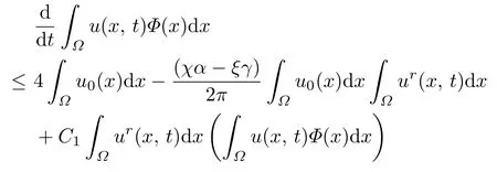
Combining the estimating I, II, III, we can obtain

Combining (4.2) with (4.3) and (4.4), we obtain that

If χα − ξγ > 0, we have that

Combining (4.5) and (4.6), this completes the proof.

Lemma 4.1Let Ω∈R2be a smooth bounded domain andx0∈Ω. Assume thatis sufficiently small, q = r, χα − ξγ > 0,and

Then the solution of(1.4)blows up in finite time.

Proof.Denote

We define

By the definition ofΦ(x) with Lemma 2.3 associated, we know

Together with the condition in Theorem 1.2(i), it is easy to find that both E(0) < 0 and E′(s) > 0 holds for s > 0. This yields E(MΦ(0)) < 0 providedsmall enough. Combining with (4.7) to get

We obtain from (4.7) and (4.8) that

This concludes that there exists a T ∈(0, ∞) such that MΦ(t)→0 as t →T. We complete the proof.

Proposition 4.2Letq > r, x0∈Ω and0 < r1< r2< dist(x0, ∂Ω)denote the distance betweenx0and∂Ω. Then there existC11, C12> 0relying onr1, r2, dist(x0, ∂Ω),such that fort ∈(0, Tmax),

Proof.From (4.2), we have that

We have from (4.3) that

By the H¨older’s inequality, one has

So, we can obtain from (4.4) and (4.12) that

By the similar proof of (4.6), if χαq − ξγr > 0, we can obtain that

Combining (4.8), (4.11), (4.13) and (4.14), we complete the proof.

Lemma 4.2Let Ω∈R2be a smooth bounded domain andx0∈Ω. Assume that is sufficiently small, q > r, χαq − ξγr > 0,

Then the solution of(1.4)blows up in finite time.

Proof.By the similar proof of Lemma 4.1, we can get the result of Lemma 4.2, and skip the proof for conciseness.

The proof of Theorem 1.2 is completed by Lemmas 4.1 and 4.2.