Modeling the carbon dynamics of alpine grassland in the Qinghai-Tibetan Plateau under scenarios of 1.5 and 2 °C global warming

YI Shu-Hua, XIANG Bo, MENG Bao-Ping, WU Xiao-Dong, DING Yong-Jian*

a Instiute of Fragile Ecosystem and Environment, Nantong University, Nantong, 226007, China

b School of Geographic Sciences, Nantong University, Nantong, 226007, China

c State Key Laboratory of Cryospheric Science, Northwest Institute of Eco-Environment and Resources, Chinese Academy of Sciences, Lanzhou, 730000, China

d Chongqing Climate Center, Chongqing, 401147, China

e Cryosphere Research Station on the Qinghai-Tibetan Plateau, Lanzhou, 730000, China

f Key Laboratory of Ecohydrology of Inland River Basin, Chinese Academy of Sciences, Lanzhou, 730000, China

g University of Chinese Academy Sciences, Beijing, 100049, China

AbstractAlpine grassland occupies two-thirds of the Qinghai-Tibetan Plateau(QTP).It is vital to project changes of this vulnerable ecosystem under different climate change scenarios before taking any mitigation or adaptation measures.In this study,we used a process-based ecosystem model,driven with output from global circulation models under different Representative Concentration Pathways (RCPs), to project the carbon dynamics of alpine grassland.The results showed the following:1)Vegetation carbon(C)on the QTP increased by 22-38 gC m-2 during periods of 1.5 and 2 °C warming under different RCPs when compared to the baseline period(1981-2006),while soil C increased by 85-122 gC m-2.2) The increases of vegetation C and soil C at the period of 1.5 °C warming were about 15 gC m-2 and 40 gC m-2 smaller than those at the period of 2 °C warming, respectively; increase of C was greater for alpine meadow than for alpine steppe. 3) Precipitation, radiation, and permafrost changed significantly and showed heterogeneous spatial patterns, and caused heterogeneous response of C dynamics. For alpine meadow in regions transformed from permafrost to seasonally frozen soil with medium annual precipitation (200-400 mm), vegetation C and net primary production decreased by 18.7 gC m-2 and 3.1 gC m-2 per year during 2 °C warming under RCP 4.5,respectively.This decrease can be attributed to the disappearing impermeable permafrost. Different from previous studies that indicated an unfavorable response of alpine grassland to climate warming, this study showed a relatively favorable response, which is mainly attributed to CO2 fertilization.

Keywords: Permafrost; Terrestrial ecosystem model; Vegetation; Soil; Net primary production

1. Introduction

Thermal and hydrological conditions are critical factors affecting ecosystem dynamics (Wang et al., 2016a; Xia et al.,2018). Climate change will affect these conditions especially for high-latitude and high-altitude regions predicted to experience “much greater than average” warming (Yang et al.,2014). Furthermore, the deepening of active layer or disappearance of permafrost of these regions also alters the thermal and hydrological regimes of the soil(Ye et al.,2009;Yi et al.,2014).Therefore,cold region ecosystems,which have already adapted to the cold environment, will experience substantial changes in the future (Wang et al., 2008; Ding et al., 2019).

Alpine grassland is the typical vegetation type and occupies 2/3 of the Qinghai-Tibetan Plateau (QTP) (Wang et al.,2016b). It provides the basis for pastoral production, water,and soil reservation. It is also considered as a fragile ecosystem and is sensitive to climate change. Therefore, projecting changes of alpine grassland under different climate change scenarios is vital to establish mitigation and adaptation measures for sustainable development.

Most studies related to climate changes on alpine grassland are based on “space-for-time” methods with in situ observation (Wang et al., 2012; Qin et al., 2014) or remote sensing dataset(Yi et al.,2011;Zhou et al.,2015;Wang et al.,2016a).Some other studies that adopted process-based model investigated climate changes on alpine grassland but did not explicitly consider the effects of permafrost on the QTP (Tan et al., 2010; Zhuang et al., 2010; Zhu et al., 2016). Yi et al.(2014) simulated the dynamics of both permafrost and alpine grassland ecosystem with a dynamic organic soil version of the terrestrial ecosystem model. However, only 1-3°C static warming was applied throughout the whole simulation to investigate the process of permafrost degradation and its impact on alpine grassland. The abovementioned studies are not suitable for projecting the changes of alpine grassland under different emission scenarios where atmospheric CO2concentration, precipitation, and radiation will change. Hence, the main aim of this study is to project responses of alpine grassland to global warming of 1.5 and 2°C above preindustrial levels and to permafrost degradation using a process-based ecosystem model driven with outputs from global climate models.

2. Methods

2.1. Model description

We used a dynamic organic soil version of the terrestrial ecosystem model (DOS-TEM) (Raich et al., 1991; McGuire et al., 1992) to simulate carbon and permafrost dynamics on the QTP (Fig.1).Two schemes were developed for the model application on alpine grassland. First, a soil skin temperature scheme was developed with a dataset from meteorological station observation and simulation using the Community Land Model(Yi et al.,2013).Bare soil surface skin temperature was measured routinely every day in a meteorological station;while soil surface skin temperature under vegetation cover was simulated using the Community Land Model. The relationships between soil surface skin temperature and leaf area index and environmental factors (e.g., air temperature and radiation) were then developed for use in the DOS-TEM. A permafrost hydrology scheme following the Community Land Model (Yi et al., 2014) was also developed to simulate the effects of permafrost degradation on soil water content.Ground water reservoir was treated as a special soil layer when the last soil layer is frozen; this prevents exchange of water between the soil layer and groundwater reservoir.However, when permafrost degrades, the exchange of water can happen, depending on matric potential and hydraulic conductivity. The parameterizations of thermal, hydrological,and ecological processes used in this study were the same as those of Yi et al. (2014); thus, Yi et al. (2014) should be referred to for more details.

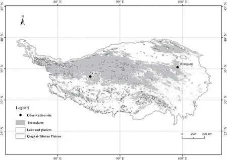
Fig.1.Spatial distribution of permafrost on the Qinghai-Tibetan Plateau(Zou et al., 2017) and locations of two observation sites for calibrating ecological parameters, Gaize for alpine steppe and Wenquan for alpine meadow (black dots).

2.2. Meteorological driving dataset

Outputs from five global circulation models (GCMs)-GFDL-ESM2M, HadGEM2-ES, IPSL_CM5A_LR, MIROCESM-CHEM, and NorESM1-M-were used. These GCMs were run under three representative concentration pathways(RCPs), i.e., RCP 2.6, 4.5, and 8.5, within the CMIP5 project(Moss et al.,2010).These dataset has been bias-corrected with the WATCH reanalysis data and downscaled to 0.5°resolution(Su et al., 2017).

Monthly mean surface air temperature and daily maximum and minimum air temperature, radiation, vapor pressure, and annual precipitation were used. We calculated the mean of each variable from five GCMs as ensemble to drive the DOSTEM.

We used the same timing of global mean temperature increase relative to 1861-1900 mean as that used in Shi et al.(2018). The threshold times of warming of 1.5°C were 2030, 2028, and 2025 for RCP2.6, 4.5, and 8.5, respectively,and those of 2°C were 2049 and 2039 for RCP4.5 and 8.5,respectively. Increase of temperature never exceeded 2°C before 2100 under RCP2.6. Both 15 years before and after each threshold time were considered in calculating the mean state of alpine grassland ecosystem for comparison.

2.3. Vegetation and soil texture

We considered two types of vegetation on the QTP, alpine meadow and alpine steppe(Zhang et al.,1988).We calculated the area fraction of each vegetation type within each 0.5°grid cell. Both vegetation types may exist in the same grid cell(Fig. 2a). We defined each different combination of climate and vegetation type as a cohort. There were 1079 cohorts altogether.

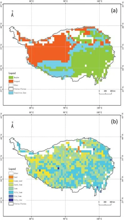
Fig.2.Spatial distribution of(a)alpine meadow and alpine steppe,and(b)soil texture.

The soil data,including the sand and clay mass fractions of the surface soil (0-30 cm) and the bottom soil (30-100 cm),were obtained from http://globalchange.bnu.edu.cn/research/soil (Shangguan et al., 2012). The soil mass fractions were resampled to 0.5°and recalculated into each soil texture according to the International Soil Texture Triangle (Fig. 2b).

2.4. Model calibration

We calibrated rate-limiting parameters (e.g., the maximum rate of photosynthesis and heterotrophic respiration rate) for each grassland type following the protocols given in McGuire et al. (1992). We used field measurement values, such as vegetation carbon and nitrogen, soil carbon, and nitrogen,from two permafrost sites, namely Gaize (33.05°N, 84.16°E,4734 m a.s.l.)and Wenquan(35.53°N,99.51°E,4260 m a.s.l.),as target values for calibrating alpine steppe and meadow,respectively(Fig.1 and Table 1).The Gaize site was primarily a steppe ecosystem in the western QTP, with the dominant plant species being Carex moorcroftii, Stipa roborowskyi,Kobresia humilis, and S. purpurea. The sampling site was located in a mountain basin, which was the main landform in the Gaize area(Wu et al.,2016).The average vegetation cover of the steppe was 15%at the sampling site.The Wenquan site was located at the eastern part of the permafrost regions on the QTP. This sampling site consisted primarily of rolling hills with valleys and basins and was primarily a typical meadow ecosystem(Wu et al.,2017).The sampling site was located in a mountain slope with a gradient of 2°. The vegetation cover was 80%, and the common plant species included Kobresia tibetica, K. pygmaea, K. humilis, C. moorcroftii, and S.roborowskyi.The vegetation carbon(VEGC),soil carbon,and nitrogen contents were measured by the quadrat method(1 m×1 m),and five plots were taken at each site during the peak growing season. Samples were collected for laboratory analysis.All these are common practices of ecological studies.Net primary production (NPP) was represented using peak above-ground biomass (Scurlock et al., 2002). The mean monthly climate data for the 1951-1980 period from the GCM grid cells corresponding to these two sites were used for calibration.

2.5. Model simulation and analysis

To investigate the effects of CO2fertilization, we ran two types of simulations: 1) using different CO2concentrations from different RCPs for the period 2007-2099 (Clarke et al.,2010), and 2) using constant CO2concentration of 380 × 10-6, which represents the average atmospheric CO2concentration for 2007-2099.

To further investigate the role of other environments on alpine grassland ecosystem, we first classified all grid cells into nine types with different combinations of annual precipitation(D:＜200 mm;W:＞400 mm;M for others)and frozen soil conditions (P: permafrost; S: seasonally frozen soil; P2S:changed from permafrost to seasonally frozen soil). The calculation period used for precipitation was 1981-2006. We defined permafrost as the last soil layer (with the bottom at 3.2 m from the surface) frozen between 1981 and the beginning of each warming period. The seasonally frozen soil was defined as the last soil layer always unfrozen during the period.Each cohort was assigned to a combination.A variable in a combination was calculated from the variable of cohorts weighted with area fraction. Finally, we analyzed the changes of ecosystem carbon between the 1.5 or 2°C global warming period and baseline period(1981-2006)under different RCPs within each combination.

The concept of active layer thickness is only valid for permafrost, which can degrade to seasonally frozen soil.Therefore, we used the maximum unfrozen thickness, which corresponds to the active layer thickness in permafrost regions and is equal to the total soil thickness (3.2 m, the part above bedrock) in seasonal frozen regions.

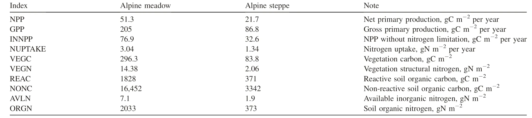
Table 1Target values for calibration of parameters in the DOS-TEM(for detailed information, please refer to McGuire et al. (1992) and Zhuang et al. (2010)).

3. Results

3.1. Climate changes on the QTP

The average of annual mean air temperature was ～-2.0(±0.39)°C during the baseline period. It increased to ～-0.37(±0.65), 1.06 (±0.92), and 2.88 (±1.06)°C during the 2090s for RCP 2.6, 4.5, and 8.5, respectively (Fig. 3a). The differences in air temperature simulated by different GCMs were largest under RCP 8.5. The average of annual precipitation was ～399.1 (±22.7) mm during the baseline period, and it increased to ～436.68 (±32.3), 461.16 (±42.0), and 487.08(±47.9) mm during the 2090s for RCP2.6, 4.5, and 8.5,respectively(Fig.3b).Downward shortwave radiation reduced from ～205.03 (±2.57) W m-2during the baseline period to～204.17 (±4.88), 202.40 (±6.12), and 198.25 (±6.77) W m-2for RCP2.6, 4.5, and 8.5, respectively (Fig. 3c). Atmospheric CO2concentration of RCP2.6 increased from 380 × 10-6at year 2006 to a maximum of 442×10-6around year 2045 and then reduced to 421 × 10-6at year 2099. That of RCP 4.5 stabilized around year 2070 and reached 538 × 10-6around 2099. That of RCP 8.5 increased dramatically and reached 936 ×10-6around 2099 (Fig. 3d).

3.2. Spatial distribution of variables at the baseline period

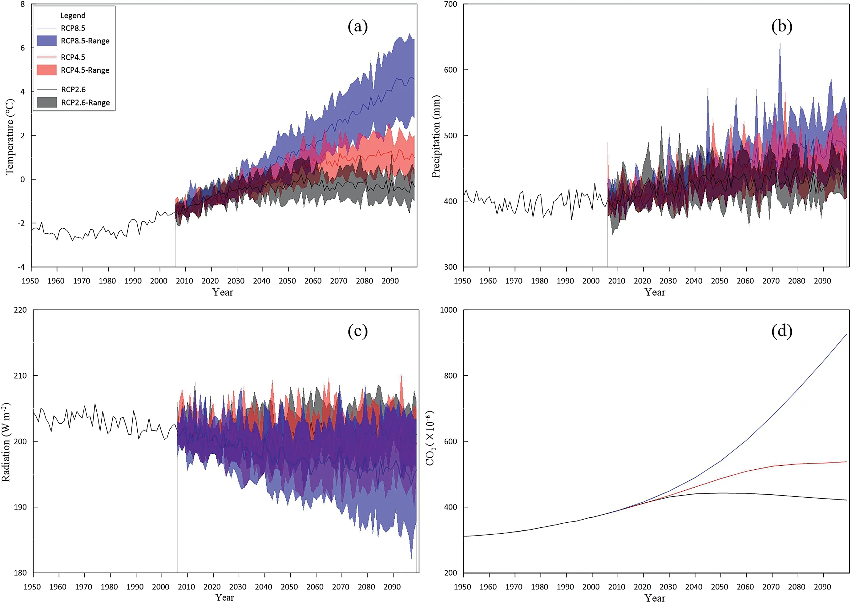
Fig.3.Changes of(a)annual mean air temperature,(b)annual precipitation,(c)annual mean radiation,and(d)annual CO2 concentration over the historical period(1950-2006) and 2006-2099 under different RCPs using ensemble mean of five GCMs (shadow area shows ± standard deviation for each variable).

During the baseline period, averages of annual mean air temperature had the lowest values of ～-10°C in the northeastern(the Qilian Mountain),central,and western parts of the QTP (Fig. 4a). Precipitation was maximized in the southeast of the QTP with more than 600 mm per year and gradually reduced to less than 100 mm per year in the northwest of the QTP(Fig.4b).On the contrary,downward shortwave radiation was minimized in the southeast, with less than 130 W m-2,and gradually increased to more than 250 W m-2in the northwest (Fig. 4c).

The simulated volumetric water content (VWC) of 20 cm was the highest in the eastern part of the QTP (Fig. 4d). The maximum unfrozen thickness was relatively small on the central part of the QTP and the eastern part of the Qilian Mountain (Fig. 4e).

The NPP was high in the central part of the QTP,but small at most of the edges(Fig.4f).Both the VEGC and soil organic carbon (SOC) were highest in the eastern part of the QTP,were minimized on the west part, and followed a similar spatial pattern of the vegetation (Figs. 4 g, h and 2a). The net ecosystem production (NEP) did not have a clear spatial pattern, with few maximums over the QTP (Fig. 4i).

The spatial patterns of these variables during the 1.5 and 2°C warming periods were similar (e.g., 1.5°C warming for RCP4.5 scenario,Fig.5).In the following section,we compare these variables for different vegetation types,different thermal and water environments, and different warming periods under the three RCPs.

3.3. Effects of CO2 fertilization

At the periods of 1.5 and 2°C global warming, VEGC respectively increased by 25.4 gC m-2and 35.6 gC m-2on average(multiyear mean for the three scenarios over all grids)when CO2fertilization was considered (Fig. 6a). In contrast,when CO2fertilization was not considered, the corresponding VEGC increased/decreased by 6.4/5.1 gC m-2(Fig. 6b).

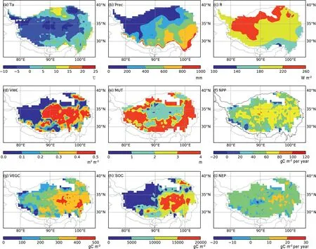
Fig.4.Spatial distribution of multiyear mean of(a)air temperature,(b)precipitation,(c)downward shortwave radiation,(d)volumetric water content at 20 cm,(e)maximum unfrozen soil thickness, (f) net primary production, (g) vegetation carbon, (h) soil organic carbon, and (i) net ecosystem production in the Qinghai-Tibetan Plateau during the 1981-2006 period.

With CO2fertilization, the NPP increased by 5.3/7.3 gC m-2per year on average at 1.5/2°C warming when compared to the baseline period (Fig. 6c). However, when CO2fertilization was not considered, NPP only increased by ～0.38 gC m-2per year at the periods of 1.5°C warming and even decreased by 2.4 gC m-2per year at the periods of 2°C warming (Fig. 6d).

With CO2fertilization, SOC increased by ～88.6/117.7 gC m-2at 1.5/2°C warming (Fig. 6e). On the other hand, SOC increased by ～55.0/15.4 gC m-2at 1.5/2°C warming without CO2fertilization (Fig. 6f).

In the following sections, we only analyze the simulations with CO2fertilization.

3.4. Changes of carbon under different RCPs

For alpine meadow, VEGC increased by ～28.8 gC m-2for 1.5°C warming under all three RCPs and ～41.1 gC m-2for 2°C warming under RCP 4.5 and 8.5 (Fig. 7a). The NPP increased by ～5.1 gC m-2per year and 7.0 gC m-2per year for 1.5 and 2°C warming under different RCPs, respectively(Fig.7c).The SOC all increased by ～111.4 gC m-2for 1.5°C warming under all three RCPs and increased by ～142 gC m-2for 2°C warming under RCP 4.5 and 8.5 (Fig. 7e). Heterotrophic respiration (RH) increased more than NPP at different warming periods under different RCP scenarios (figure not shown). Therefore, the NEP decreased by ～1.8 gC m-2per year and ～2.9 gC m-2per year for 1.5 and 2°C warming,respectively, where the decrease under RCP 8.5 was greater than that under RCP4.5 (Fig. 7g).

For alpine steppe,VEGC increased by ～22.0 and ～29.9 gC m-2for 1.5 and 2°C global warming, respectively (Fig. 7b).The NPP increased by ～5.5 gC m-2and ～7.6 gC m-2per year for 1.5 and 2°C global warming under different RCPs(Fig.7d). The SOC increased by ～62.0 and ～92.6 gC m-2for 1.5 and 2°C warming, respectively (Fig. 7f). The NEP decreased by ～0.79 gC m-2per year for 1.5°C warming under RCP2.6 and decreased by ～0.15 and ～0.45 gC m-2per year for 1.5 and 2°C warming under RCP4.5, respectively. The NEP increased by ～0.98 and ～0.73 gC m-2per year for 1.5 and 2°C global warming under RCP8.5, respectively(Fig. 7h).

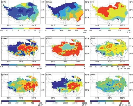
Fig. 5. Same as Fig. 4, but for the case of 1.5 °C warming using RCP4.5 scenario.

3.5. Changes of carbon and environment for alpine meadow

Since the spatial patterns of various carbon and environment variables were similar among different RCPs and at different warming periods, for the following analysis, we chose the simulation at 2°C warming period under RCP 4.5.The majority of alpine meadow were distributed in the S-W(seasonally frozen soil regions-wet) region, P2S (permafrost to seasonally frozen soil transition)-W region, and P2S-M(medium wet) regions with fractions of 46.9%, 14.8%, and 8.3%, respectively (Fig. 8a). The P-D and P2S-D only accounted for ～0.2% and ～1.1% of the total number of grids,respectively (Fig. 8a). In the following analysis, we did not include alpine meadow in the P-D and P2S-D regions.

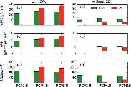
Fig.6.Differences in multiyear means of(a-b)vegetation carbon(VEGC),(c-d)net primary production(NPP),and(e-f)soil organic carbon(SOC)between the period of 1.5/2 °C global warming under different RCPs and the baseline period (1981-2006) with and without CO2 fertilization effect.

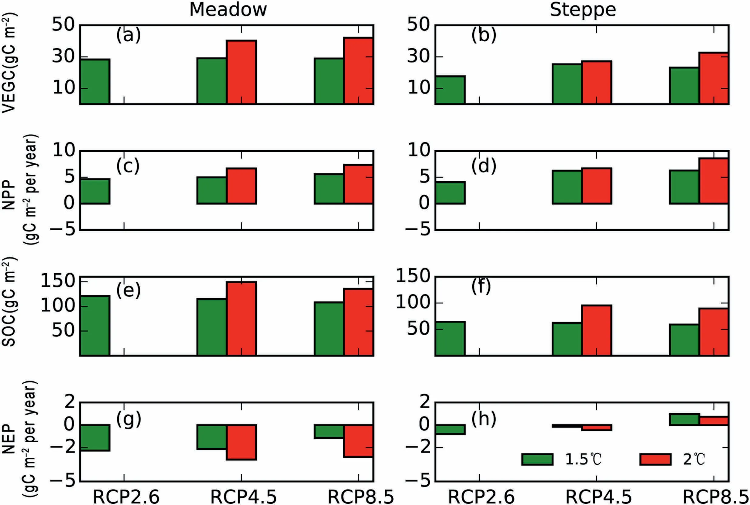
Fig.7.Differences in multiyear means of(a-b)vegetation carbon(VEGC),(c-d)net primary production(NPP),(e-f)soil organic carbon(SOC),and(g-h)net ecosystem production(NEP) between the period of 1.5/2 °C global warming under different RCPs and the baseline period(1981-2006)for alpine meadow and steppe.

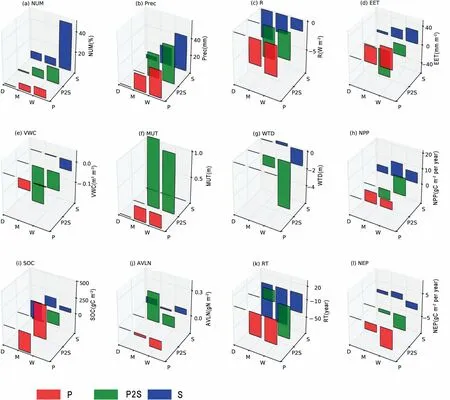
Fig.8.The(a)number fraction of grid cells,difference of multiyear mean of(b)annual precipitation,(c)shortwave radiation,(d)evapotranspiration,(e)volumetric water content at 20 cm,(f)maximum unfrozen thickness,(g)water table depth,(h)net primary production,(i)soil organic carbon,(k)available nitrogen,(k)soil organic carbon residence time,and(l)net ecosystem production between the period of 2 °C global warming under RCP4.5 and the baseline period(1981-2006)for alpine meadow at regions with different combinations of permafrost state, e.g., permafrost (P), without permafrost (S), and vanishing permafrost (P2S), and precipitation, e.g., ＜200 mm (D), ＞400 mm (W), and others (M).

Precipitation increased when compared with the baseline period with the highest precipitation on the wet regions (W;～44.6 mm per year; Fig. 8b). Radiation all decreased with an average of ～3.6 W m-2(Fig. 8c). The majority of the regions showed increased evapotranspiration (EET, Fig. 8d), except for the P2S-M regions.The VWC decreased in several regions,with the largest being ～0.18 in the P2S-M region (Fig. 8e).Maximum unfrozen soil thickness (MUT) increased the most in the P2S regions (Fig. 8f). Water table depth (WTD)decreased the most in the P2S-W regions of ～5.39 m, which indicates movement of water from soil into water reservoir(Fig. 8g). The NPP generally increased with the exception of the P2S-M region (～6.2 gC m-2per year; Fig. 7h). The SOC decreased by more than 276 gC m-2in the S-D and P-M regions and increased by ～606 gC m-2in the P-W region(Fig.8i).Available nitrogen(AVLN)increased the most in the P2S-M region (Fig. 8j). Residence time decreased for most regions by 15%-24%, which suggests increased carbon exchange (Fig. 8k), while it increased by 9.7% in the P2S-M region. Changes of NEP increased in most regions but decreased by ～6.5 gC m-2per year in the P2S-M region(Fig. 8l).

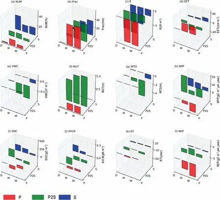
Fig. 9. Same as Fig. 8, but for alpine steppe.

3.6. Changes of carbon and environment for alpine steppe

Alpine steppe was distributed the most in the S-D regions,with 29.2%, and the least in the P-D regions, with 1.6%(Fig. 9a). In the following analysis, we did not include alpine steppe in the P-D region.

Changes of precipitation were similar to those of alpine meadow (Fig. 9b), but the amount of increase was smaller.Radiation reduced the most on the permafrost regions and dry regions (Fig. 9c). The VWC decreased the most on the P2S-M and P2S-W regions for ～0.11 m3m-3and～0.13 m3m-3, respectively (Fig. 9e). The NPP and VEGC increased the most in the dry regions. They decreased by～10.3 gC m-2and 35 gC m-2per year in the P-W regions,respectively (Fig. 9h). The SOC showed a pattern similar to those of NPP and VEGC (Fig. 9i). Available nitrogen increased the most in the S-D region of ～0.16 gN m-2and decreased the most in the P2S-D region of ～0.16 gN m-2(Fig. 9j). Residence time changed slightly over all regions(Fig. 9k). The NEP decreased by ～10.2 gC m-2per year in the P-W region and increased by ～21.0 gC m-2per year in P2S-D region (Fig. 9l).

4. Discussion

4.1. Effects of permafrost degradation on surface soil water

Previous hydrological studies on basins with permafrost have demonstrated that permafrost degradation will cause draining of soil water into groundwater (Ye et al., 2009; Niu et al., 2011). It is hypothesized that surface soil water content,which is an important limiting factor of alpine grassland growth (Baumann et al., 2009), will reduce, which will adversely affect vegetation growth.However,the degradation process is slow and cannot be detected easily without comprehensive long-term observation. The processes of exchange between soil water and groundwater have been implemented in few ecosystem models(Zhuang et al.,2010).Yi et al. (2014) simulated the exchange of soil water and groundwater following the method of Community Land Model version 3.5 (Swenson et al., 2013). Unfortunately, the comparisons among the control run and runs with 1, 2, and 3°C warming were for over 100 years. The effects on shallow soil water content become minimal.In this study,we compared the warming period and the baseline period. More soil water drained into groundwater, and the water table depth became shallower in wet regions than in medium wet regions when permafrost disappeared for both alpine meadow and alpine steppe (Figs. 8g and 9g). Shallow soil water content also reduced in these regions. These reductions can be attributed to the draining of soil water into groundwater,since precipitation increased and evapotranspiration decreased or increased in small amounts (Figs. 8b-e and 9b-e). It is obvious for alpine meadow that reduction of shallow soil water content was the major cause of reduction of NPP and VEGC (Fig. 8h).

4.2. Complex responses of vegetation growth under global warming

Environmental changes under a warming world involve more than increase of air temperature. Under different RCPs,CO2concentration, precipitation, and radiation changed, and these changes showed large spatial heterogeneity (Figs. 3, 8 and 9). Previous studies mainly focused on the adverse effects of warming but neglected other beneficial effects,such as lengthening of growing season, CO2fertilization, more precipitation, and less radiation, which reduces evapotranspiration. As shown in this study, CO2fertilization played a dominant role in fixing more carbon into the ecosystem(Fig.6),which is consistent with the result of Piao et al.(2012)and Ding et al. (2017). The Special Report also demonstrated that “increase of ecosystem respiration might be countered by enhanced CO2concentration and higher temperature with medium confidence (Hoegh-Guldberg et al., 2018). As shown in Figs. 8 and 9, the changes of precipitation, radiation,permafrost degradation, and water exchange between soil and ground water were heterogeneous on the QTP, which caused heterogeneous responses of carbon dynamics.Taking the QTP as a whole, both VEGC and soil carbon increased in 1.5 and 2°C global warming periods under different RCPs.

4.3. Uncertainties and limitations

Yi et al. (2014) simulated an increasing trend of VEGC over a period of 1982-2012 on the west of the QTP;however,the normalized difference vegetation index from satellite observation showed no increasing trend. It is suggested that driving climate dataset, gravel content, and erosion process,which were not implemented in the modeling study, might be the major reasons(Yi et al.,2014).We also simulated a similar trend in this study (figures not shown here). We used a different climate driving data from the Climate Research Unit dataset of Yi et al. (2014). Therefore, the similar trend might not be caused by the driving climate dataset.

We simulated an increase of NPP and VEGC in the dry regions for alpine steppe in the warming periods under RCPs(Fig.9h).However,the precipitation and soil water content did not increase.At both warming periods and the baseline period,surface soil water contents were close to 0.01 m3m-3, which is the minimum water content prescribed in the DOS-TEM.We cannot attribute the increase of VEGC to environmental changes for alpine steppe of the dry regions. The DOS-TEM performance in dry regions should be improved in the future.

Although we successfully simulated the effects of permafrost degradation on soil water and then on vegetation growth,there are several uncertainties relating to this process.We used a total of 3.2 m soil layers above bedrock and defined the disappearance of permafrost when the last soil layer was unfrozen in summer. This might not be realistic, especially as there are larger amounts of ground ice well below 3.2 m(Wang et al., 2018). We also do not know when soil water starts to exchange with groundwater, which is a very complex process (Cheng and Jin, 2013). Cooperation with the groundwater research communities will help to reduce the associated uncertainties.

Another uncertainty comes from the atmospheric driving dataset.As shown in Fig.3,air temperature,precipitation,and solar radiation had large differences among five different GCM outputs.The differences increased with time.Therefore,for further studies,researchers should use ensemble dataset by averaging multiple GCM outputs (Fang and Li, 2016). However, it would be better to drive the DOS-TEM with each individual GCM output for evaluating the uncertainties associated with the driving dataset in the future.

5. Conclusion

We simulated the carbon dynamics of alpine grassland on the QTP and assessed the changes at both 1.5 and 2°C global warming periods under different RCPs. Such assessments cannot be performed using field observation and have not been performed in previous modeling studies. Alpine grassland on the QTP as a whole showed an increase in both VEGC and soil carbon for all cases, mainly due to CO2fertilization. Without CO2fertilization effects,constraint of air temperature increase by 1.5°C will cause more absorption of atmospheric CO2by grassland ecosystem than of 2°C. The pattern changed when CO2fertilization effects are considered. In addition to air temperature and atmospheric CO2concentration, other environmental conditions, such as precipitation, radiation, and permafrost, changed significantly and showed heterogeneous spatial patterns,and caused heterogeneous response of carbon dynamics. In this study, we identified the effect of permafrost degradation process on vegetation growth. Permafrost degradation, indicating the disappearance of the impermeable layer for water infiltration, will result in a decrease of soil water availability for plant growth, which will further lead to vegetation degradation.

Conflict of interest

The authors declare no conflict of interest.

Acknowledgments

We thank Ms.LU Meng-Xia and HUANG Yu-Ting,and Dr.LYU Yan-Yan for editing of this manuscript. This study was jointly supported through grants provided as part of the National Natural Science Foundation of China (41690142,41730751), and the State Key Laboratory of Cryospheric Science (SKLCS-ZZ-2-2018).