A generalized model for estimation of aerodynamic forces and moments for irregularly shaped bodies

Elvedin Kljuno, Alan Catovic

Mechanical Engineering Faculty, University of Sarajevo, Vilsonovo setaliste 9, 71000, Sarajevo, Bosnia and Herzegovina

Keywords:Aerodynamic force Aerodynamic moment Fragments

A B S T R A C T A novel method for estimation of an aerodynamic force and moment acting on an irregularly shaped body(such as HE projectile fragments)during its flight through the atmosphere is presented.The model assumes that fragments can be approximated with a tri-axial ellipsoid that has continuous surface given as a mathematical function. The model was validated with CFD data for a tri-axial ellipsoid and verified using CFD data on aerodynamic forces and moments acting on an irregularly shaped fragment.The contribution of this method is that it represents a significant step toward a modeling that does not require a cumbersome CFD simulation results for estimation of fragment dynamic and kinematic parameters.Due to this advantage,the model can predict the fragment motion consuming a negligible time when compared to the corresponding time consumed by CFD simulations. Parametric representation(generalization)of the fragment geometrical data and the conditions provides the way to analyze various correlations and how parameters influence the dynamics of the fragment flight.

1. Introduction

Complete aerodynamic characteristics generally do not exist for the potentially wide variety of body shapes. For the calculation of the body trajectory, apart from the data on projected (exposed)surface area of the body,velocity data and data on the density of the fluid through which the body is moving,one needs also the data on the values of aerodynamic force and aerodynamic moment acting on the body at any given moment.Values of force and moment are crucial in the calculation of fragment trajectory and its movement through the air.

It is not practical for each potential shape of a body to determine the values of aerodynamic forces and moments using numerical simulations (CFD), so it is useful to define a generalized model to estimate the values of total aerodynamic force and aerodynamic moment acting on a body with an arbitrary shape. Examples of irregularly shaped bodies are:

- primary fragments made after the detonation of high explosive projectiles (natural or controlled fragmentation), missiles,bombs;

- primary and secondary fragments originating from improvised explosive devices (IED);

- splinters formed after the rupture of various structures(different materials) due to the effects of severe storms (tornadoes and hurricanes, for example, both contain strong rotating winds that can cause significant damage);

- primary and secondary fragments resulting from the explosion of ammunition storage sites;

- meteoroid bodies coming from outer space.

Generally, most objects in nature are irregularly shaped, so the usefulness of this model (in regard of estimation of a trajectory,velocity, energy, and stability of these bodies) could be significant for many areas of research.Usually,determination of force,required for calculation of body center of mass trajectory (there is no mentioning of moment coefficients in the literature),is done using aerodynamic force coefficients. These coefficients (coefficients of total aerodynamic force components) are usually determined analytically or experimentally.

Twisdale in his work [1] used cross-flow theory in order to analytically estimate the aerodynamic coefficients for a uniformly random spatial orientation of the body, knowing the aerodynamic coefficient values for precisely defined directions of the body with continuous geometry. This approach has been used earlier to develop the wind axis aerodynamic forces as a function of an angle of attack for slender cylinders knowing only the drag force coefficients for the body in normal flow to the major body axes[Hoerner, 1965]. Twisdale in his paper [1] presents cross-flow aerodynamics for rectangular parallelepipeds (approximation of irregularly shaped body),where for different parallelepiped lengths(slenderness ratio), drag, lift and side force coefficients are estimated as a function of attack and roll angle, using analytical expressions, where different corrective factors (skin friction and aspect-ratio correction) are also used. It is not explained in the paper how the exposed area of a body is determined for an arbitrary orientation of a body. Based on the value of the drag, lift and side force coefficients,and using the values of dynamic pressure and the reference area of the body, a total aerodynamic force is estimated.

In the previous work [2], experimental methods for estimating drag force coefficient values are explained in more detail.As far as experimental data is concerned, the first thing to notice in the literature is that there is no experimental data on aerodynamic lift coefficients for bodies with irregular shapes.Furthermore,one of the disadvantages noticed is that most of the experimental tests contain very little data on the drag coefficients values in the supersonic regime. Another disadvantage is that no (available) experimental research has given specific details of how the exposed surface of fragments is determined,as well as the data on dimensions and the mass of fragments. These data significantly affect the drag coefficient values obtained in experimental tests.

Most experimental tests for determination of drag coefficients for irregularly shaped bodies were conducted in the period from 1955. to 1995., and no data are available on whether more recent tests have been conducted with modern data acquisition equipment. Some researchers [McDonald,1980)] state that the drag coefficient in the subsonic and supersonic flow is assumed constant,which in reality is not the case, and it is probably a certain approximation of the drag coefficient,due to the lack of data.Other researchers in their papers indicate that the drag coefficient for fragments can be taken as a constant for all velocities [Crull 1998,Zehrt 1998,Swisdak 2005],arguing that the fragments in the initial phase of their trajectory move at speeds up to several times higher than the local sound velocity. However, the drag coefficient depends on the shape of a body,as well as its velocity,and coefficient variation may have a significant effect on body trajectory,a fact that is rarely emphasized in the literature. Generally speaking,the task of estimation of aerodynamic forces and moments acting on a body of an irregular shape is quite complex since they do not have a continuous surface. For this reason, in our model, a tri-axial ellipsoid was used as a shape that can best approximate an arbitrary body shape of different dimensions.This model is,also,a follow up on our previous work where the exposed area of the irregularly shaped body is estimated.Both of these models will be further used in our next paper,where the model for estimation of a trajectory for a body with an irregular shape will be presented.

In this model,irregularly shaped body geometry can be defined parametrically,and it is possible in a very short amount of time(in a matter of seconds)to estimate the values of total force and moment acting on these bodies. This is significant advantage of a model,comparing it to the method of determination of aerodynamic force and moment using CFD methods.

In summary, the model developed in this paper represents a generalized model for bodies of an irregular shape,because,based on the initial conditions, and only knowing the shape of the fragments, the necessary calculations of forces and moments can be performed.

In available literature, no similar model for estimation of aerodynamic forces and moments for the irregularly shaped body was found, so our model presents significant step towards better understanding of flight dynamics of irregularly shaped bodies.Fig.1 shows the major steps of the estimation.

2. Physical model

An irregularly shaped body can be approximated with a tri-axial ellipsoid, using the same method described in the earlier related paper on the estimation of projected surface area of an irregularly shaped body [2]. Fig. 2 gives a schematic representation of the ellipsoid body surface with a fluid flowing around it with velocity v→.The normal vector for the surface dA is marked with n→,and the angle between the velocity vector and the normal vector is denoted by δ.

Fig.3 shows a schematic model of a fluid element collision with the fragment surface, which authors find suitable after analyzing the flow field (CFD simulations [3,4]) around the fragment (and making a kind of analogy with a set of rigid bodies collision with massive obstacle and their interaction after the collision) where it was noticed that streamlines generally leave the surface in a tangential direction,due to the fluid elements interaction.Here,the output velocity vector vizl→is perpendicular to the normal vector n→(shown in Fig.3)and it is in the same plane with vectors vul→and n→.Since fluid elements interact with each other immediately after striking the surface of the body, then their paths correspond to those shown in Fig. 3, i.e. the fluid flows around the body. This assumption is used to calculate the change in the momentum of fluid elements colliding with the surface,which provides the way to estimate the overall resistance force of the fragment.

Newton's Second Law may be written in the following form

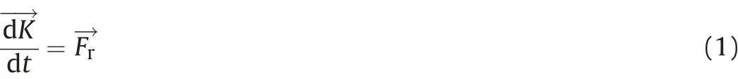
then the change of momentum vector can be expressed as

For a normal vector on the surface of an ellipsoid (further explanation on this formula can be found in Appendix 1, and in details in Ref. [2]), we can write

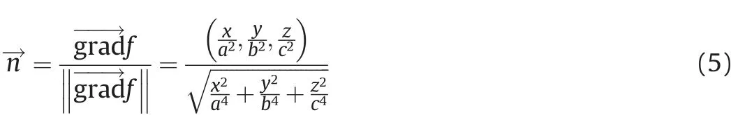
Fig. 3 shows (because of the orthogonality of the vectors)

Also,the following is valid(because the vectors vul→, vizl→and n→are in the same plane)

The following can also be written(by dividing the input velocityvul→into the components v⊥→and v||→in the direction of tangent and normal on the surface of the ellipsoid)

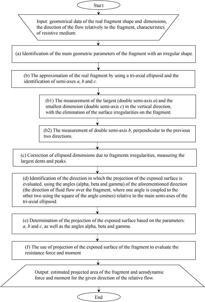
Fig.1. The flowchart of the estimation process of the resistance force and moment.

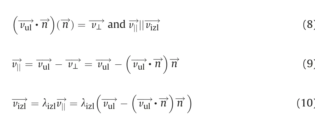
In (8) vul→·n→represents the projection of input velocity vector onto a normal,which,together with normal unit vector n→,gives a component of input velocity (v⊥→) in the direction of normal. According to the continuity equation, on the surface of the body following condition must be satisfied

So, together with vizl0→(the unit vector in the direction of the output vector vizl→) and (10), the following can be written

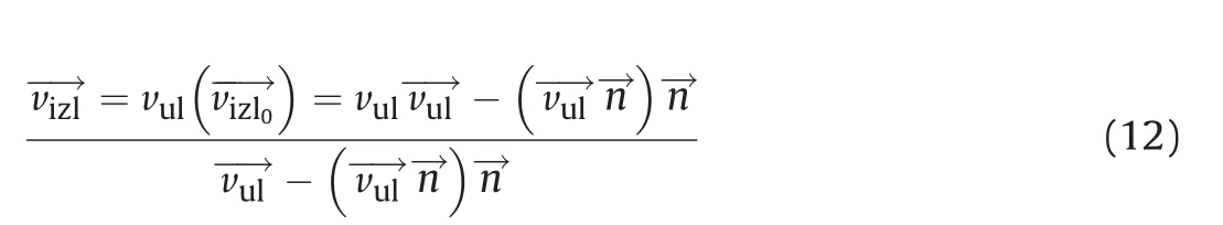
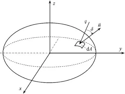
Fig. 2. Representation of the ellipsoid body surface with a fluid flowing around it.

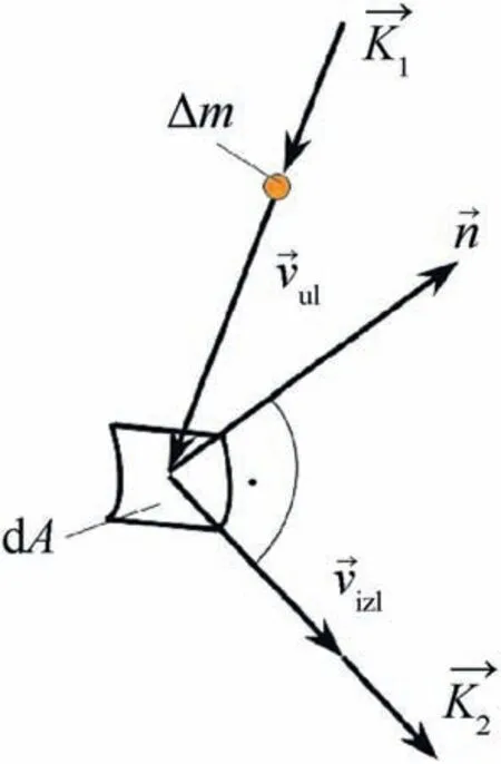
Fig. 3. The momentum change due to the collision with the fragment surface. Output velocity vector vizl→is perpendicular to the normal vector n→. Input velocity is represented with vector.vul→

where v is the inlet velocity magnitude.The expression(14)in the denominator can be presented in the following form

where

In (14), the inlet velocity is.Fig. 4 shows the schematic projection of the elemental surface dA, perpendicular to the velocity vector direction. This projected elemental surface is shown in Fig. 4 as ΔAp. Fig. 4 also shows the resultant force for the element dA on the ellipsoidal surface.For the elementary mass (Fig. 4), it can be written

The total aerodynamic force acting on the body can be presented in the form

In (20)the formula for output velocity vizl→is given by(14).The negative sign in(19)is used because we want to determine how the fluid acts on the fragment,not the other way around as presented in initial setup of the model.However,the momentum change law is written for the fluid element and the derived force is used to obtain the integral resistance force acting on the fragment.

In (19) and (20) Aexpis exposed surface area of the ellipsoid above the closed curve cexp, shown in Fig. 5. Therefore, the integration will be carried out over the planeshown in Fig. 6) to which the axis ζ is perpendicular (Fig. 5), over the area limited by curve cexp.

For curve cexpthe following can be applied (further details on these formulas can be found in Appendix 1,and in detail in Ref.[2])

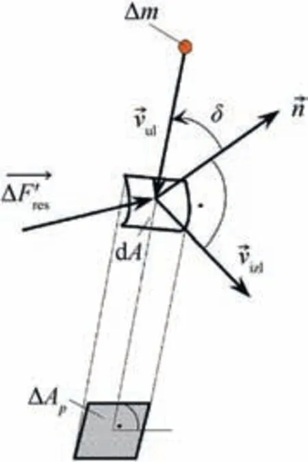
Fig.4. Schematic projection of the elemental surface dA,perpendicular to the velocity vector direction (the subscript “izl“ denotes outlet, and “ul” denotes inlet).

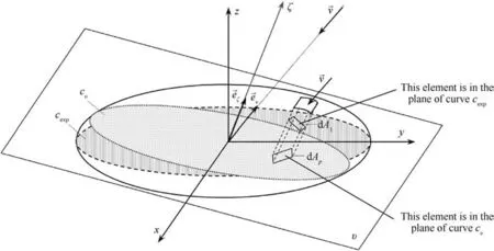
Fig. 5. Schematic representation of the parameters used to determine the aerodynamic force.

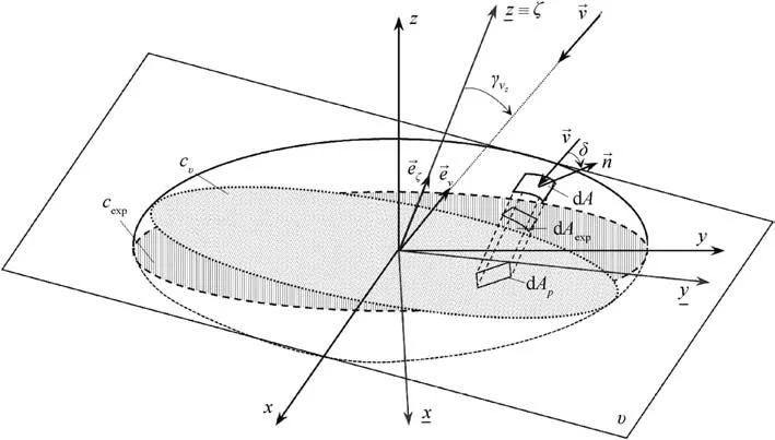
Fig. 6. Rotation of the coordinate system.

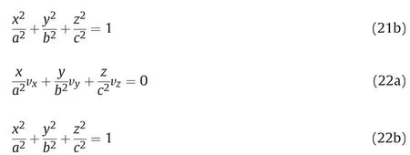
Fig.6 shows the rotation of the xyz coordinate system in order to obtain axyz coordinate system in which one axis (z≡ζ) is perpendicular to the plane in which the curve cexp is located and the other two axes (x andybelong to that plane.

For the curve cexp, also, the following applies (Fig. 6)

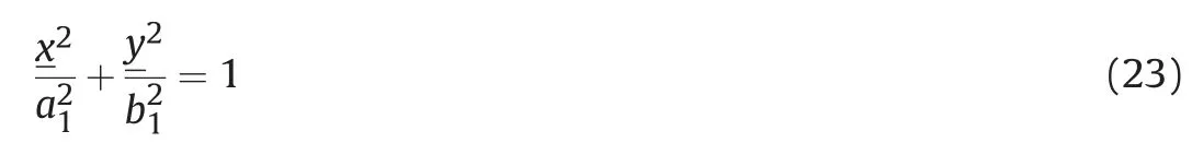
where a1and b1are semi-axes of an ellipse in the plane in which curve cexplies(Fig.6).These axes are determined according to the procedure described in our paper on the assessment of the projected surface area of the body [2]. Summarized details of this model are presented also in Appendix 1.

For projected surface dApwe can write

where, cosγvz=·

If(23)and(24) are inserted into(20),the following is obtained

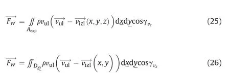
It should be noted that in(25)there are two coordinate systems(xyz andIt is necessary to decide over which variables to integrate in (25) and to express all other variables with them.

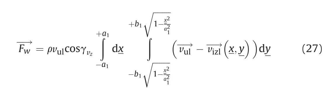
Finally, we can write an expression for the total aerodynamic force y in the projection plane Rv,and the boundary of the integration is defined,using the curve(ellipse) Cexp.

Using expressions derived in our previous paper on the assessment of the projected surface area of the body [2] (Summarized details presented in Appendix 1)for x,y and z coordinates,the coordinates of the projection point P (see Fig. 7) in the “old” xyz coordinate system are

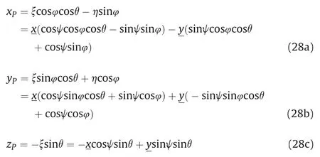
where the integration is done using the coordinatesx and

Now,from the projection point P we need to find the point C at the surface(the ellipsoid),which represents the intersection of the perpendicular line passing through the projection point P at the projection plane and the ellipsoidal surface (see Fig. 7).

This is done in the reverse order (starting from the projection point and then finding the point at the surface of which P is the projection point), because the overall integration of the force is transferred to the projection plane Rv(The integration is done usingandcoordinates,since the boundary of the integration is defined within this plane Rv,using the curve Cexpand projecting it onto the projection planeRv. For further details about the described coordinate transformation, see Appendix 1 and ref.[2]).

In(25)the coordinatesx and y(in the plane Rv)are involved,and the x,y and z coordinates for calculating the gradients and normal on the surface at a given point of ellipsoid defined by x, y and z in the“old”coordinate system are to be used.Fig.7 shows a schematic way of solving this problem.

In the essence, first the projection plane of an ellipsoid,perpendicular to the velocity vector, is found (plane Rυ, Fig. 7).When solving the double integral in(27),using numerical methods,the plane Rυ is numerically divided, and then we search for points on the ellipsoidal surface that have a projection on that plane.

The radius vector of point C on the ellipsoid surface, shown in Fig. 7, can be presented as

where rp→=- the radius of the point p - projection of an arbitrary ellipsoid point C to the plane Rυ (perpendicular to the velocity vector v→), and d→- the vector of distance between these two points in the direction of the velocity vector.

In (29), r→must satisfy the following condition

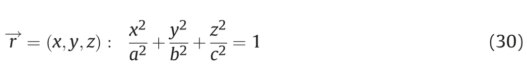
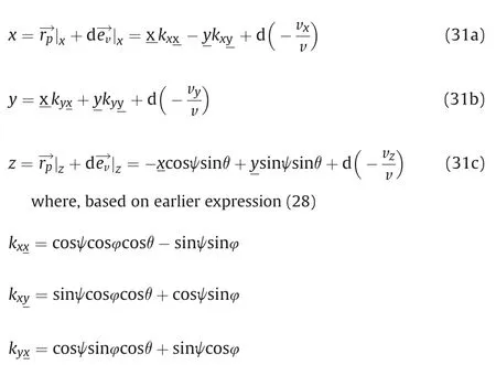
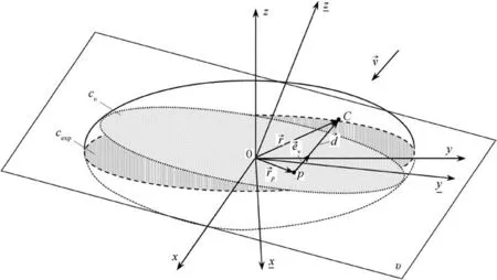
Fig. 7. The procedure of searching the point C on the ellipsoid surface, corresponding to the projected point P in the transformed coordinate system.

So, with the help of the vector d→, we look for a point on the ellipsoid surface corresponding to the projected point in the transformed coordinate system

Within this physical model, the goal was also to establish a model for prediction of the aerodynamic moment acting on an irregularly shaped body during its flight through the atmosphere.The aerodynamic moment estimate relies on the aerodynamic force estimation method, previously described.

Generally speaking, the aerodynamic moment can be represented in the differential form ass a differential aerodynamic force acting on the differential segment on the surface of the body (Fig. 6), and r→- the position vector of the differential element on the surface of the body.

The differential aerodynamic force is defined by the expression

where

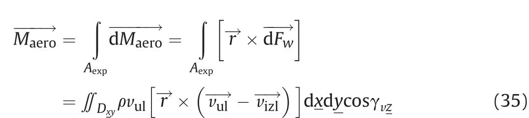
Using the differential of the force, the total aerodynamic moment is determined by (33)

Cexp- an ellipse that separates the front (exposed) part of the ellipsoid from its end part, relative to the velocity vector (Fig. 6).

In order to carry out the estimation of aerodynamic forces and moments according to the developed physical model,a program in Matlab was written, and given in Appendix 2.

This model is an important step towards modeling that does not require numerical simulations(CFD)to estimate aerodynamic force and moment. Using this model, in conjunction with the model for estimating the projected surface area of the body[2],the fragment trajectory can be estimated in a simpler way (compared to the calculation in CFD programs)because the force and moment can be estimated very fast for every orientation of a body, and in every moment of its trajectory.

With the developed model for aerodynamic force and moment,the required parameters are obtained within a few seconds, while the use of numerical simulations to evaluate the aerodynamic force and moment values takes more than 12 h(in our case,a computer with following components was used:AMD Ryzen 7(8 CPU cores,8 Threads)at 3 Ghz,16 GB of RAM and a Radeon RX 580 graphics card with 36 calculation units and 8 GB of GDDR5 memory).

3. Validation of the physical model

The developed physical model was validated using the data for aerodynamic force and moment obtained from numerical simulations of air flowing around a tri-axial ellipsoid, shown in Fig. 8.

Semi-axes of an ellipsoid with which the validation of the developed model was performed were as follows: a=0,034m,b=0,00865m and c=0,006m.These dimensions of ellipsoid were selected because the fragment with which the numerical simulations(CFD)were performed was of similar dimensions(maximum dimensions in three mutually perpendicular directions).Directions of the coordinate system axes(attached to the center of the mass of an ellipsoid)are shown in the lower left corner of Fig.8,and also in Fig. 9.

Fig. 9 shows numerical mesh around an ellipsoid for which numerical simulations were performed.

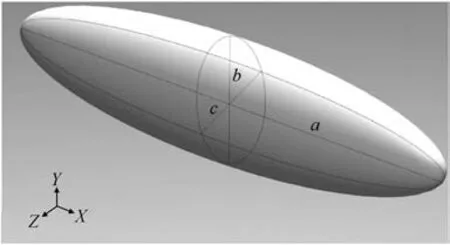
Fig. 8. Schematic representation of an ellipsoid with which validation of a model for estimation of aerodynamic force and moment was performed.

Fig. 9. Numerical mesh around an ellipsoid for which numerical simulations were performed.The method of numerical simulations of air flow around an ellipsoid consisted of the:- digitalization of the body model (3D model in Solidworks, exported to Fluent),- domain discretization (consisting of around 1,5 million cells),- characterization of the resistive medium,- initial and boundary conditions,- solver and turbulence model selection, and- aerodynamic force and moment components estimation (postprocessor).

The body was considered stationary and the flow around it was analyzed. Numerical simulations for several ellipsoid orientations were performed for angles 0°-90°with 15°angle increments. The velocity vector was directed in the positive direction of axis z,and of the coordinate system set in the body center of mass(Figs.8 and 9).

For all body orientations,simulations of flow over the body for 8 different velocities (0.6, 0.8, 1, 1.2, 1.3, 1.5, 2, and 3 Mach) were carried out (in total, 56 simulations, where every simulation needed around 12 h for convergence, using earlier mentioned computer). In numerical simulations air is modeled as homogeneous, isotropic,ideal gas.

At the end of the domain, Pressure Farfield condition was used, which is often used where the compressibility is significant. The No Slip condition is defined on the surface of the ellipsoid, which means that the relative flow velocity on the surface of the body is equal to zero. Boundary condition (The Wall) is generally used in the case when the viscous effects cannot be ignored and is relevant to most fluid flow situations.Density-based solver was selected in the simulations, where mass, flow, and energy equations are determined as the Navier-Stokes equation system in integral form for an arbitrary control volume. The Spalart-Allmaras turbulence model was used also in the simulations. This physical model of turbulence has been developed specifically for aerodynamic applications and has proven to be effective for the boundary layers with high-pressure gradients, and has been very effective for transonic flows around the aero profiles, including flows with significant separation of the boundary layer.

Methodology for numerical simulations is similar to the one used in our previous paper [3,4], so we didn't give a detailed description of it in order to avoid overlaps.The main difference is in the geometry, so here, instead of a fragment, we run numerical simulations for a tri-axial ellipsoid (for purpose of model validation).

Table 1 shows the comparison of results for the aerodynamic force acting on the ellipsoid (presented Figs. 8 and 9), obtained by Ansys Fluent numerical simulations, with the results for aerodynamic force obtained using the physical model described in this paper.

Table 1 shows data for the airflow in the direction of z-axis(ellipsoid rotation was performed around the x-axis, Fig. 8). The different orientation of the ellipsoid corresponds to the different angular increment (from 15°) of the ellipsoid obtained by rotation around the x-axis.

Generally speaking, Table 1 shows that there is no extreme deviation (relative differences were from 0,04% to around 88%) of the force values obtained by numerical simulations with the values obtained using the developed physical model, and the obtained force values are of the same order of magnitude.

Table 2 compares the results obtained by CFD numerical simulations and the developed physical model for the aerodynamic moment acting on the ellipsoid(shown in Fig.8).As in the case of aerodynamic forces, in Table 2 data on the aerodynamic moment were also given for an airflow (velocity vector direction) in the direction of z-axis(ellipsoid rotation performed around the x-axis,as shown in Fig. 8).

It should be noted that in Table 2 the aerodynamic moment values were not given for the ellipsoid orientation of 0°and 90°because the aerodynamic moments in this ellipsoid position are equal to zero (center of mass for ellipsoid lies, due to body symmetry, on z-axis for given initial conditions). In this case (Table 2),the relative differences for aerodynamic moments between 2,8%and 73,8% were recorded.

Although these relative differences (Tables 1 and 2) may seem significant at first glance, one should bear in mind the simplicity and efficiency of the developed model, the initial assumptions in the model, the complexity of the problem and the speed of calculation using the developed model(a few thousand times the speed of the force and moment calculation in numerical simulations).

The basic assumptions of the developed model for estimating aerodynamic force and moment are:

- The irregularly shaped body surface is approximated by a triaxial ellipsoid with a continually exposed surface.

- Fluid elements after impact on the surface of the body have an output velocity in the direction of the tangent to the surface,in the plane which contains the normal and the direction of the fluid input velocity.

- Pressure does not change significantly locally in the vicinity of the elemental surface of the body.

- Based on the local aerodynamic force acting on a body surface element,it is possible to determine the local pressure,which can be used to determine the local density ρ,assuming the adiabatic compression and corresponding equation of the adiabatic change.However,the density then has an influence on the local momentum change, which is the basis for calculation of the local (elementary) aerodynamic force. This means that the procedure should be done iteratively.

- Fluid compression is adiabatic because of relatively high velocities of the body so that the time constants of the local compression (the time when the fluid element enters from the undisturbed state into the compression zone around the body and then leaves the zone) are relatively small compared to the time constants of the heat transfer dynamics.The most important reasons for the deviation of model results from the results obtained with numerical simulations could be a summary effect of the following:

- Complete integration of the control volume around the body is not performed in the calculation.

- Classical equations of fluid mechanics(Navier-Stokes equations)are not solved in the model.

- The most significant deviations generally occur when the exposed surface has a relatively high curvature (i.e. a small radius of the elemental surface) because the assumption that the fluid elements remain on the surface and continue to move in the direction of the tangent is ignored, thereby eliminating the possibility of separating the local streamlines from surface on the exposed side of the body.

- Tangential stresses due to the viscosity were ignored because the air is modeled as an ideal gas so only the normal stresses were used in calculations.

- Air compressibility was not taken into account in the model.

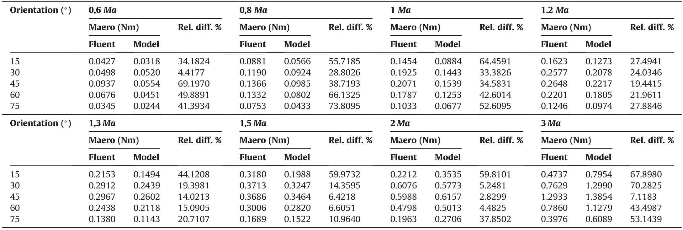
Table 2Comparison of results for the aerodynamic moment acting on an ellipsoid,obtained by simulations and developed model(airflow in direction of the z-axis,rotation around the x-axis).

4. Application of the model to an irregularly shaped body(fragment)

After the validation of the physical model, the results of the model for estimation of aerodynamic force and moment were compared (verified) with the results obtained by CFD numerical simulations for aerodynamic forces and moments acting on an irregularly shaped fragment(shown in Fig.10).

In order to determine the values of the components of the aerodynamic force and moment, the CFD numerical simulations(for different velocities of the compressible, turbulent, steady flow around the irregularly shaped fragment) were performed in the Ansys Fluent CFD package for fragment in different orientations (0°-90°, with 15°angular increments in each simulation separately). As in the case of an ellipsoid, simulations were performed for eight different velocities (0.6, 0.8,1,1.2,1.3,1.5, 2, and 3 Mach).

Methodology of numerical simulations for fragment are the same as ones used in our previous paper[3,4].For the sake of clarity and to avoid overlap between different research papers, here we only present results (aerodynamic forces and moments) for different axis of fragment rotation and different airflow axis.

As an additional comparison in our work, in Fig.11 and Fig.12 we present obtained pressure and velocity flow field, as well as streamlines(in one plane)around an ellipsoid and a fragment with an irregular shape.Both bodies have the same semi-axes a,b and c.Airflow was in this case in the direction of x-axis, with a flow velocity of 2 Ma.

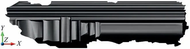
Fig.10. CAD model of fragment.

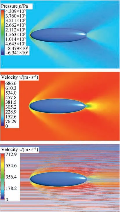
Fig. 11. Pressure and velocity flow-field, as well as streamlines around an ellipsoid(airflow in direction of x-axis, 2 Ma velocity).

Generally speaking,flows around irregularly shaped high-speed bodies are always viscous and compressible, with dominant pressure force,strong shock waves with large pressure gradients,large temperatures, turbulent flow, unsteady flow fields, and often by separating the boundary layer from the surface of the body. Main sources of the flow resistance to a moving body are practically three natural phenomena: fluid viscosity, shock waves (generally at speeds larger than 1 Ma),as well as turbulence and vortices behind the body.

In a relatively slender position of a body (airflow direction was towards x-axis,with the smallest exposed area of body,Figs.11 and 12) there is no significant separation of the airflow. The turbulent flow behind the body is smaller and the resistive force is predominantly due to viscous friction in boundary layer.By comparing flow fields around an ellipsoid and a fragment(Figs.11 and 12),one can immediately notice the disturbance in the flow around the fragment due to its irregular shape,sharp edges,dents,and surface discontinuities (stochastic shape).

This irregularity of fragment shape causes the formation of a number of smaller shock waves along its surface (Fig. 12). The appearance of these side shock waves leads to a local increase in the drag force. Furthermore, behind fragment (Fig.12.) there is larger flow recirculation zone comparing to the flow around an ellipsoid(Fig.11).Also,fragment exhibits bow shock with a larger radius and larger underpressure zone behind it, increasing total drag force.

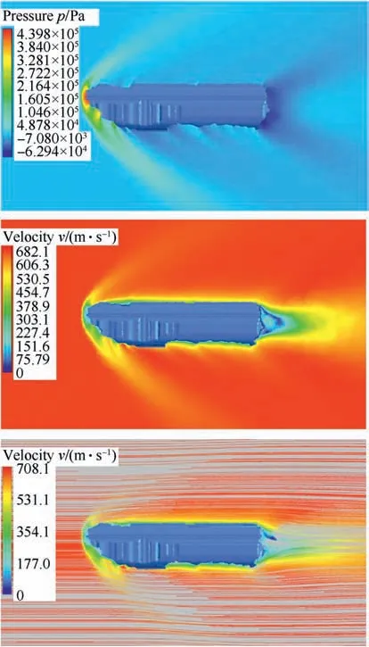
Fig.12. Pressure and velocity flow-field, as well as streamlines around an irregularly shaped fragment (airflow in direction of x-axis, 2 Ma).

In Fig.13 and Fig.14 we present obtained pressure and velocity flow-field,as well as streamlines(in one plane)around an ellipsoid and fragment, but this time airflow was in direction of z-axis (towards the largest exposed area of these bodies), with a flow velocity of 2 Ma.In relatively blunt position of a body(airflow in z-axis direction,Figs.13 and 14)pressure gradients increase significantly.The pressure gradient on the upper surface becomes so large that there is a separation of the flow which leads to the reduction of the pressure on the back and the recirculation of the flow with the vortices that dissipate part of the mechanical energy and thus increase the total drag force.

Generally, vortices are usually in mutual interaction, they are movable and can exchange energy. That is why pressure drag increases, and when the body is exposed to fluid flow through its larger surface,the pressure drag is much higher than the frictional drag.

As expected for the supersonic flow (Figs.13 and 14), there is significant overpressure zone in front of bodies,while behind them there is a region of underpressure, which also leads to increase in drag force. When comparing the flow field around these bodies,regarding streamlines(Figs.13 and 14),it can be seen that fragment(Fig.14) exhibits larger vortices and bigger recirculation area than an ellipsoid(Fig.13).Also,the underpressure area is slightly larger in the case of a fragment.

Table 3 shows the comparison of results for the aerodynamic force acting on the fragment(Fig.10),obtained by CFD Ansys Fluent numerical simulations with the results for aerodynamic force obtained using the physical model described in this paper. Table 3 shows data for the airflow in the direction of z-axis (fragment rotation was performed around the x-axis, Fig. 10). Table 3 also shows that a relative difference between the models varied from 11,1%to 96,8%,and the obtained force values are of the same order of magnitude,which is remarkable result since we are dealing with irregularly shaped body.

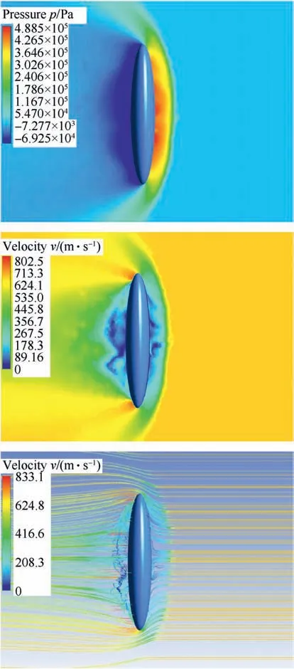
Fig. 13. Pressure and velocity flow-field, as well as streamlines around an ellipsoid(airflow in direction of z-axis, 2 Ma velocity).

Table 4, on the other hand, compares the results obtained by numerical simulations and the developed model for the aerodynamic moment acting on a fragment (Fig. 10). Data on the aerodynamic moment were given also for airflow in the direction of z-axis (fragment rotation performed around the x-axis, Fig.10).

In this case, the relative differences between 3,7% and 152,5%were recorded. These results, considering the assumptions, limitation, and simplicity of our model, are also satisfactory.

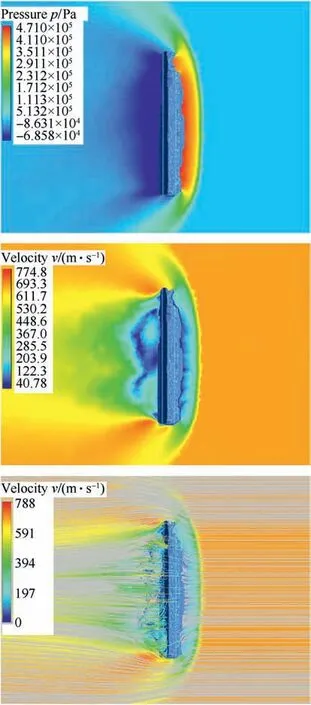
Fig.14. Pressure and velocity flow-field, as well as streamlines around an irregularly shaped fragment (airflow in direction of z-axis, 2 Ma).

Overall, considering the developed model significantly optimizes computer processing time and resources, and considering the constraints and limitations of the model, the obtained results for aerodynamic force and moment are satisfactory.The significant advantage of this model, compared to the classical approach (numerical simulations), is the overall possibility of generalization by identifying certain geometric parameters of an irregularly shaped body (a, b, c semi-axes, i.e. geometric ratios a/b and a/c), and the generalization of flight mechanics of an arbitrary shaped body,which cannot be done through classical approach using numerical simulations.

The developed model for estimating aerodynamic force and model, described in this paper, can be used, together with a developed model for estimating the projected surface area of the body [2], for predicting all relevant kinematic parameters of an irregularly shaped bodies during their motion through the atmosphere (trajectory, translational and angular velocities, translational and angular accelerations,orientation in an arbitrary time,etc.).

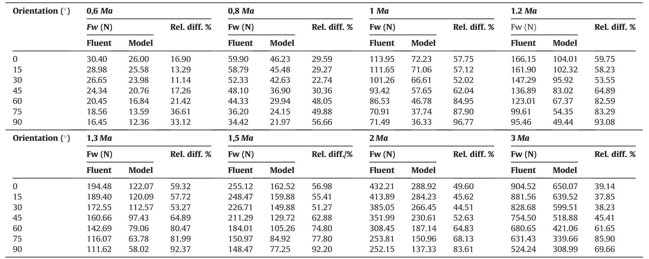
Table 3Comparison of results for the aerodynamic force acting on a fragment,obtained by simulations and developed model(airflow in direction of the z-axis,rotation around the xaxis).

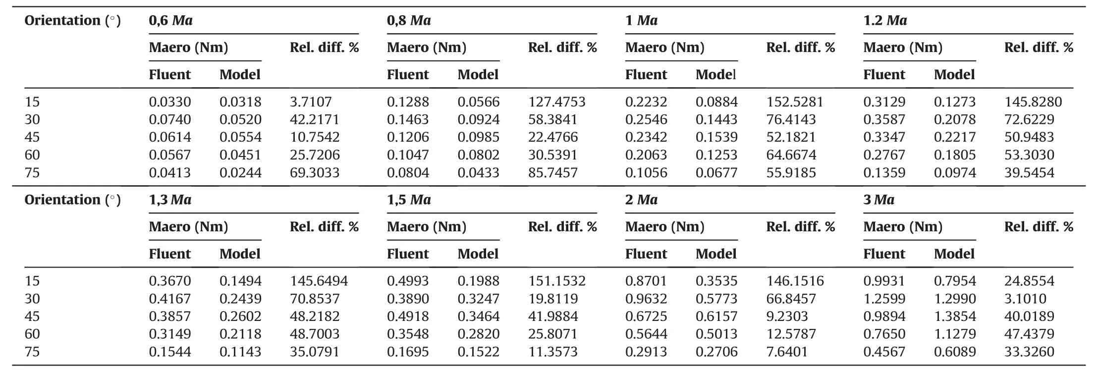
Table 4Comparison of results for the aerodynamic moment acting on a fragment,obtained by simulations and developed model(airflow in direction of the z-axis,rotation around the x-axis).

5. Conclusions

A new method for prediction of an aerodynamic force and moment for an irregularly shaped body (approximated with a triaxial ellipsoid) is developed.

The model was validated with CFD data for a tri-axial ellipsoid and verified using CFD data on aerodynamic forces and moments acting on an irregularly shaped body (HE projectile fragment).

Comparison between CFD force data and force data obtained from developed model show for an irregularly shaped body (HE projectile fragment) a relative difference from 11% for some orientation and velocity up to maximal 97% for other orientation and velocity.Obtained force and moment values were of the same order of magnitude which is satisfactory result since the estimation of dynamic parameters of an irregularly shaped body is very complex phenomena.

This method represents a significant step toward a modeling that does not require a CFD result for estimation of fragment dynamic and kinematic parameters.

Advantages of this model over classical approach (numerical simulations) are:

(1) The possibility of generalization by identifying geometric parameters of an irregularly shaped body(semi-axes a,b and c or their ratios).

(2) Significant optimization of computer processing time(several thousand times faster calculation than using numerical simulations).

(3) The model can be used,together with a model for estimating the projected surface area of the fragment[2],for predicting all relevant kinematic parameters of an irregularly shaped body during its motion through the atmosphere.

The results (aerodynamic forces and moments) obtained with the model presented in this paper could be used to integrate the equations of motion. So, the next step in the research will be the development of a generalized model for the estimation of all relevant kinematic parameters (trajectory, velocities, orientation) of irregularly shaped body.

Appendix A1. Determination of projected surface area of an irregularly shaped fragments

The model assumes that the fragments are approximated using the tri-axial ellipsoid. An ellipsoid has three pair-wise perpendicular axes of symmetry which intersect at a center of symmetry,called the center of the ellipsoid. The line segments that are delimited on the axes of symmetry by the ellipsoid are called the principal axes.If the three axes have different lengths,the ellipsoid is said to be tri -axial, and the axes are uniquely defined.

Fig. A1shows a tri-axial ellipsoid approximating the fragment(modeled in 3D Studio Max). Semi-axes of the ellipsoid, a, b, c are half the length of the principal axes.They correspond to the semimajor axis and semi-minor axis of an ellipse. Dimension a is the largest, and c the smallest.

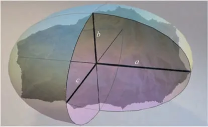
Fig. A1. Approximation of the fragment with a tri-axial ellipsoid

The projection Apof the exposed part of the surface(Fig.A2)can be presented as

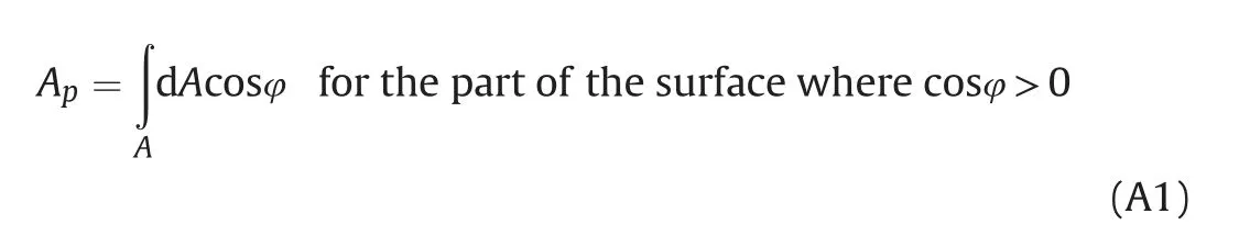
The condition on the angle means that only one(upper)part of the surface area is considered (Aexp). The upper exposed surface area has cosφ ＞0,the back of the fragment has cosφ ＜0 and on the dividing line cosφ = 0, since the orthogonal direction on the surface is perpendicular to the velocity direction v→,i.e. n→⊥v→(n→·v→=0).

Although the enclosing the integral in expresson(A1)is possible(over the closed surface A of the fragment), which allows the conversion to a volume integral using the Gauss-Ostrogradsky formula, it is not a convenient method since div（e→v）=0 because e→v≠f（x,y,z）,i.e.the projections from both sides are with opposite signs and the integral over the closed surface cancels out.Since the upper and lower part have the same projected area Ap, but the projections are with opposite signs, then

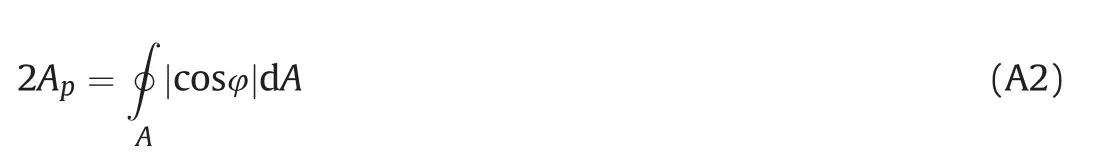
Fig. A3 shows ellipsoidal surface and projection of its element dA on the plane perpendicular to the velocity vector v→.Vector e→vis a unit vector in the line of the velocity vector (but in the opposite orientation), and the vector n→is a unit vector of the orthogonal direction to the surface dA.

Fig. A2 gives a schematic view of the convex surface and plane(normal to the velocity vector)on which the elemental surface dA is projected.The unit vector of the velocity direction is denoted by e→vand the unit vector of the orthogonal direction onto the surface element is denoted by n→.Generally, the unit vector of the normal can be obtained as

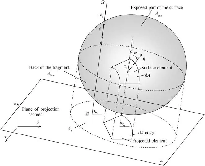
Fig. A2. Projection of surface elements (schematic view)

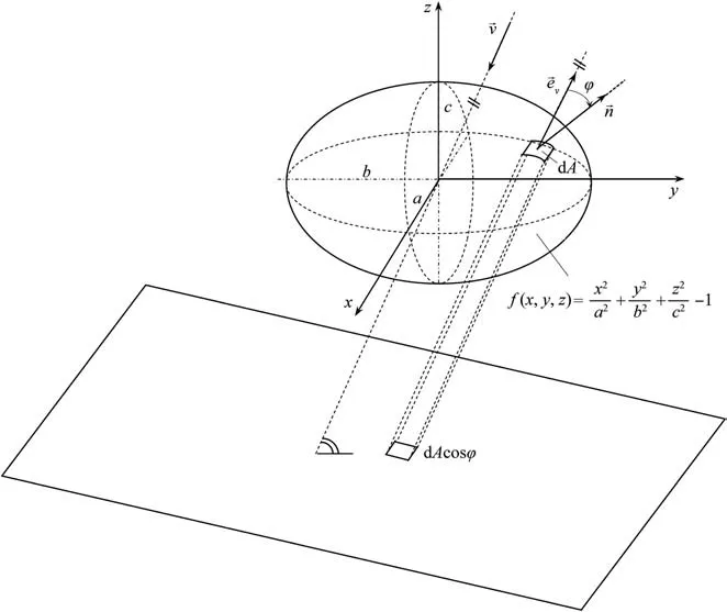
Fig. A3. Projection of ellipsoidal surface element dA on the plane perpendicular to the velocity3

The term‖grad→f‖in(A3)is the norm of gradient of f,where the gradient is in the direction of normal to the surface f.The gradient can be obtained based on the function f

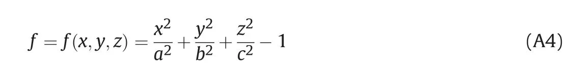
in the following form

The unit vector of the velocity direction

Angle φ (Fig. A3) is defined as an angle between unit vector n→and velocity vector,so the projection of the surface element on the plane perpendicular to the velocity vector is defined using angle cosine

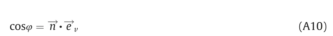
Based on (A5)

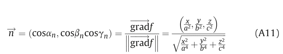
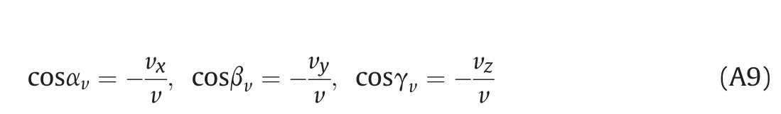
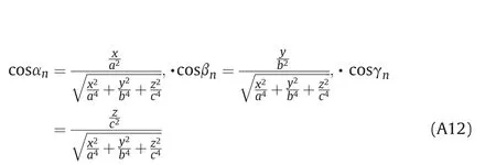
where αn,βnand γnare angles between the unit vector of normal and coordinate axes. Based on (A11)

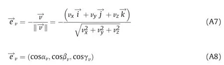
where angles αv,βvand γvare angles between the velocity vector and coordinate axes. Based on (A7) and (A8)

Using (A1), (A2), (A10), (A11) and (A12)

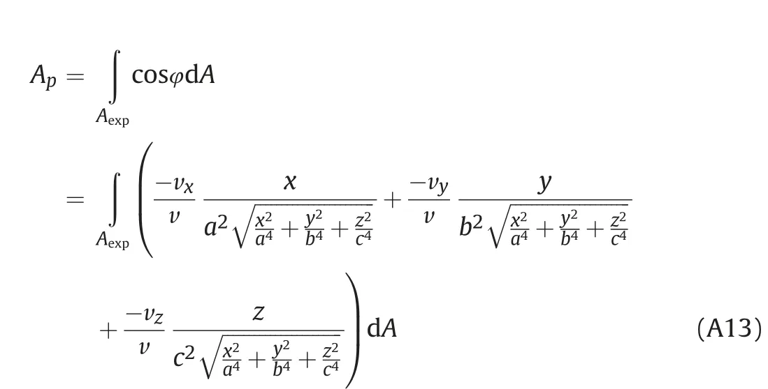
Fig. A4 shows schematically the method for determination of the curve c⊥that separates exposed surface (upper part of an ellipsoid or a first part of the incoming surface in the direction of vector velocity) from the rest of the ellipsoid. Velocity vector is perpendicular to curve c⊥in its every point,which means that unit vector n→is also perpendicular to the velocity vector.

The idea here is to find the surface limited by curve c⊥(which lies in a plane that is generally not perpendicular to the velocity vector) and then this surface should be projected on a plane (the plane π in Fig.A4)perpendicular to the velocity vector.In this way,the required projection of the complete ellipsoid that the“viewer”sees from the direction of the velocity vector is obtained.

For curve c⊥, the following applies

Based on Expression (A17)

Fig. A5 shows rotation of coordinate system xyz in order to obtain coordinate system ξηζ where one axis(ζ)is perpendicular to the plane where the curve c⊥is, and other two axes (ξ and η)belong to this plane.

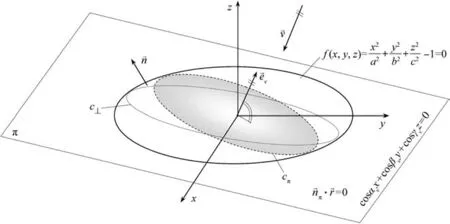
Fig. A4. determination of the curve that separates exposed surface from the rest of the ellipsoid

Curve cπrepresents an intersection of the plane π and ellipsoid.It can be written as

In Expression(A14) n→π is the unit vector of normal on the plane π, and r→is the radius vector in the plane π. From(A14)

Along with (A15), the curve cπalso satisfies the equation of ellipsoid

Fig. A5. Rotation of coordinate system xyz in order to obtain coordinate system ξηζ

For c⊥(Fig. A5), similarly as in Fig. A4,following applies

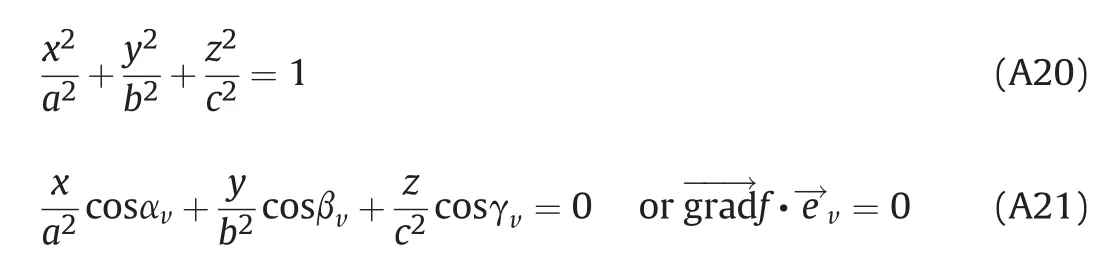
Based on Expression (A21),a vector of the normal on the plane where curve c⊥is located can be defined as

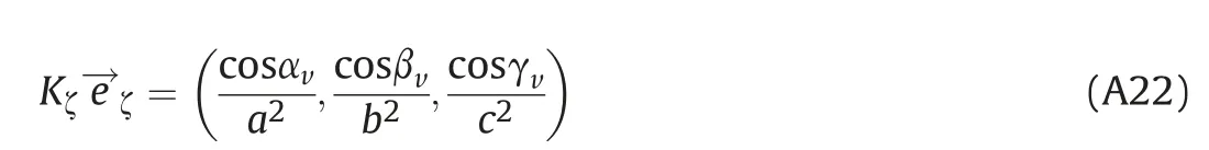
Based on Expression(A22),unit vector of normal e→ζis obtained(in this case it represents the unit vector of axis ζ) and this vector can be determined by dividing Expression(A22)with its magnitude

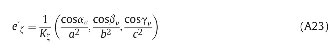
For unit vector e→ζof coordinate axis ζ generally applies

where cosαζ=cosβζ=and cosγζ=

In order to find rotation angle φ, unit vector e→ζcan be divided into two vectors e→ζxyand e→ζzas

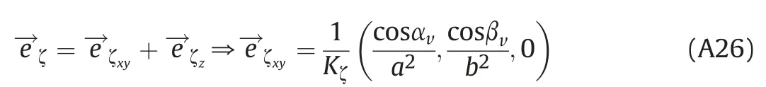
where e→ζxyis the projection of a vector e→ζon xy plane,and vector e→ζzis a component of a unit vector e→ζin the direction of z axis.Components of a vector e→ζcan be obtained using projections of a vector e→ζxyon the axes. This way we can set up relations from which we can obtain angleφ

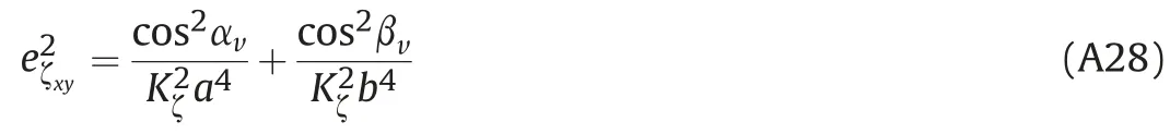
Based on (A27) and (A28) we get

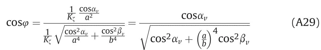
Angle γζbetween axis ζ and z axis can be determined using the component of a unit vector e→ζin the direction of z axis.The cosine of this angle represents component of a unit vector e→ζ and this component is also given with (A26), so

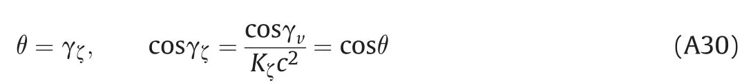
After determination of rotation angles of a coordinate system ξηζ in relation to old coordinate system xyz, it is possible to transform coordinates, i.e. express old coordinates using new coordinates

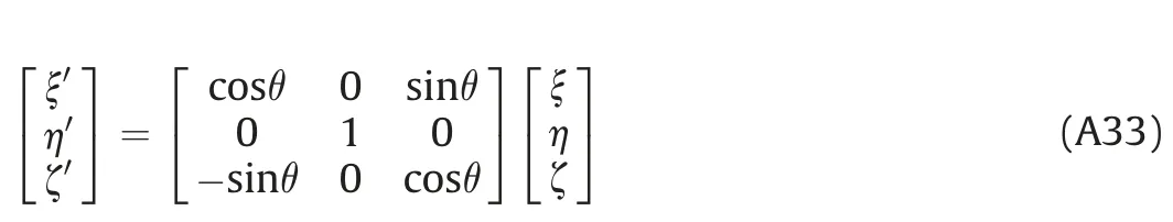
The goal is that in expressions we have the new coordinate of a rotated coordinate system. After the rotation around z axis for angle φ, we get temporary coordinate system ξ′η′ζ′where ζ′≡z,because we have rotation around z axis. The relation between coordinates can be expressed in matrix form

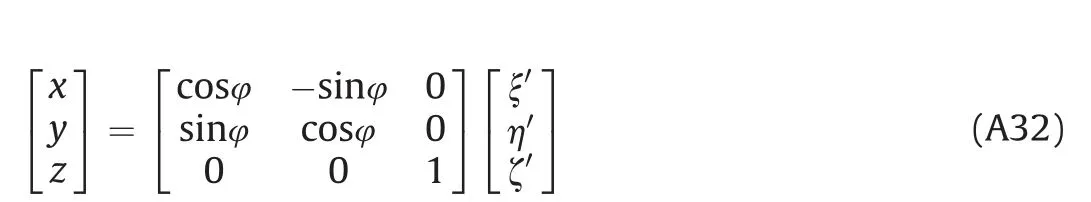
where matrix represents rotation matrix for the case of rotation around z axis. Next rotation is rotation of temporary coordinate system ξ′η′ζ′around axis η′for angle θ = γζ, so appropriate connection between coordinates is

The resulting transformation of coordinates after the two rotations is given as

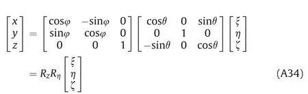
where the matrix of the two transformations of coordinates from ξηζ into xyz is

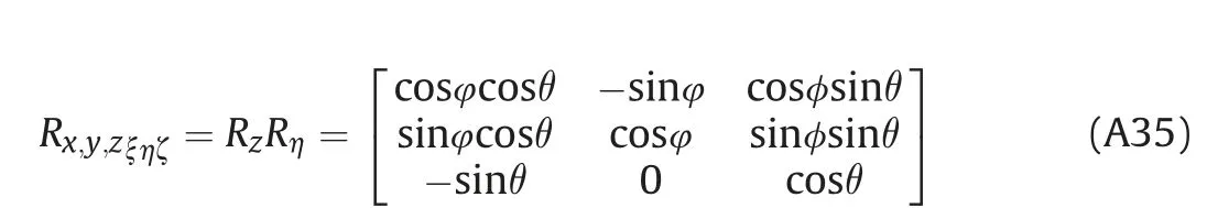
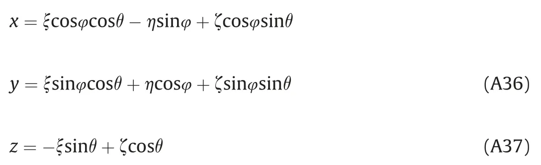
Based on (A35), we get

For the curve c⊥expressed inside the coordinate system ξηζ,expressions (A36), (A3) and (A20) apply.

ζ=0 (closed curve c⊥is in a plane ξη) (A37)

Expression (A36) can be simplified as

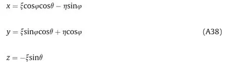
When we substitute(A38) into(A20), we obtain

which can be expressed as

In order to eliminate the part of (A40) next to 2ξη, we need to rotate coordinate system(Fig. A6).

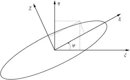
Fig. A6. Rotation of the coordinate system to eliminate the part of Expression(A40) next to the term2ξη.For the coordinate system from Fig. A6 following applies

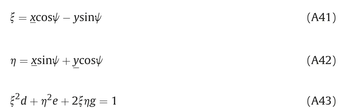
In (A41-A43)

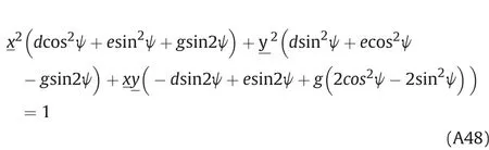
We can introduce following substitutions in (A48)

In order to eliminate the part of (A48) next towe can write

Area enclosed by the curve c⊥(which separates the exposed part of the surface from the back part of the fragmental surface)can be written as

which represents a projection of the fragment surface onto the plane containing the curve c⊥and the final formula for projected area on the plane perpendicular to the velocity vector is

where the angle φvζ is the angle between the velocity vector direction and the direction perpendicular to the plane of the dividing line c⊥.

In(A56), following parameters are involved

By combining (A41-A46), we get

Parameters d,e and g are given by(A44-A46),and angles φ and θ are given by(A29) and (A30), respectively.

Appendix 2 - MatLab program for estimation of the aerodynamic force and moment for an arbitrary body shape.