Long-time Dynamics for Thermoelastic Bresse System of Type III

2019-05-15FuNa

Communications in Mathematical Research 2019年2期

Fu Na

(School of Mathematics,Southwest Jiaotong University,Chengdu,610031)

Communicated by Wang Chun-peng

Abstract:This paper considers the thermoelastic beam system of type III with friction dissipations acting on the whole system.By using the methods developed by Chueshov and Lasiecka,we get the quasi-stability property of the system and obtain the existence of a global attractor with finite fractal dimension.Result on exponential attractors of the system is also proved.

Key words:Bresse system,quasi-stability,global attractor,fractal dimension,exponential attractor

1 Introduction

In this paper,we consider a semilinear thermoelastic Bresse system of Type III

for x∈(0,L)and t>0,with the initial conditions

where the past history function ϑ0on R+=(0,+∞)is a given datum,and the boundary conditions are as follows:

where φ,ψ,ω,θ represent,respectively,vertical displacement,shear angle,longitudin displacement and relative temperature.The coefficients ρ1,ρ2,ρ3,b,k,k0,k1,δ are positive constants related to the material and the parameter l stands for the curvature of the beam.The function g1,g2,g3are nonlinear damping terms,the functions f1,f2,f3,f4are nonlinear source terms,and h1,h2,h3,h4are external force terms.Elastic structures of the arches type are object of study in many areas like mathematics,physics and engineering.For more details,the interested reader can visit the works of Liu and Rao[1],Boussouira et al.[2]and reference therein.

Throughout the paper,the assumptions are always made as follows.

•f1,f2,f3,f4are nonlinear source terms.Assume that there exists a non-negative C2function F:R3→R such that

and there exists a constant Cf>0 such that

Furthermore,assume that F is homogeneous of order p+1,

Since F is homogeneous,the Euler homogeneous function theorem yields the following useful identity:

By(1.5),we derive that there exists a constant CF>0 such that

Assume that there exists a non-negative C2function¯F:R→R such that

and there exists a positive constantsuch that

with p≥1.

and there exists a constant κ∈(0,1)and mf>0 such that

•gi(i=1,2,3)is damping term satisfying

where mi,Mi>0 are constants.

• The memory kernel ξ(s)∈ C1(R+)is a nonnegative differentiable function such that

There exists a positive constantµsuch that

The original Bresse system is given by the following equations(see[3]):

where N,Q and M denote the axial force,the shear force and the bending moment,respectively.These forces are stress-strain relations for elastic behavior and given by

where G,E,I and h are positive constants.

In recent years,the asymptotic properties of Bresse systems(1.16),i.e.,when the fourth equation of system(1.1)is omitted,have been widely investigated(see,e.g.,[2],[4]–[9]and the references therein).They pointed out that the exponential stability of the associated solution semigroups is highly in fluenced by the structural parameters of the problem.In particular,Ma and Monteiro[5]investigated a semilinear Bresse system.They obtained the Timoshenko system as a singular limit of the Bresse system as l→0.The remaining results are concerned with the long-time dynamics of Bresse systems.They proved the existence of a smooth global attractor with finite fractal dimension and exponential attractors as well by using the methods developed by Chueshov and Lasiecka[10].They also compared the Bresse system with the Timoshenko system,in the sense of the upper-semi-continuity of their attractors as l→0.

Currently,several results on the stability properties of simplified versions of the thermoelastic system(1.1)are available in the literature,for instance regarding Timoshenko-type system where the longitudinal motion is neglected(see[11]–[15]).On the contrary,the picture concerning the full model accounting for longitudinal movements is essentially poorer.

Actually,there are some results in the literature where the authors consider Fouriertype thermal dissipation,see,e.g.,[1]and[16],and also with non Fourier-type thermal dissipation,see,e.g.,[17]and references therein.But for the thermoelastic Bresse system with Green-Naghdi-type thermal dissipation,that is,when the fourth equation of system(1.1)is replaced by the classical parabolic heat equation

Said-Houari and Humadouche[18]have recently analyzed the thermoelastic Bresse system with Green-Naghdi-type thermal dissipation.They proved that the decay rate of the solution.However,no results have been obtained for long-time dynamics.Thus,the goal of this work is to investigate the long-time dynamics of the Bresse system.

In order to exhibit the dissipative of the system(1.1),we use the transformation(see[19])

with a function χ := χ(x)satisfying

Then we get from(1.1)–(1.3)(by writing for simplicity,θ instead of˜θ)

for x∈(0,L)and t>0,with the initial conditions

and the boundary conditions

The rest of this paper is organized as follows.In Section 2,we state the result on existence and global well-posedness of the system by using classical semigroup methods.In Section 3,we find a strict Lyapunov functional to show the existence of a gradient system structure.In Section 4,we present a new definition of quasi-stability and prove that the dynamical system owns the quasi-stable property.Finally,we make our conclusions in Section 5.

2 Well-posedness

In this section,we prove that(1.17)–(1.19)can be yield a dynamical system.Let(·, ·)0and ∥·∥0be the usual inner product and norm of L2(0,L).

By virtue of the memory with past history,system do not correspond to autonomous system.To deal with the memory,motivated by[11],[20]and[21],we define a new variable η=ηt(x,s)by

Therefore the past history of θ satisfies

where ηt(0)=0 in Rn,t≥ 0,and initial condition η0(s)= η0(s)in Rn,s ∈ R+,with

By using(2.1)and(1.14),we have

Combining with(2.2)we get the following system,which is equivalent to problem(1.17)–(1.19):

for x∈(0,L)and t>0,without loss of generality k1−l0=1,with the following initial data

and the following boundary conditions

We define following weighted space with respect to the variable η,

which is a Hilbert space with the norm

and the inner-product

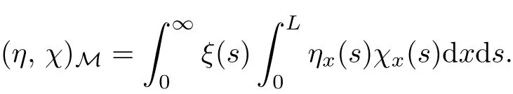
Let L=(L2(0,L))4.Define the inner product of L as

for any v=(v1,v2,v3,v4)∈L and,and its induced norm as

Set H=H×L×M,whose inner product and induced normal are as

2.1 Energy Inequality

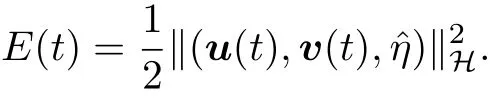
In this subsection,we give the energy inequality.The linear energy of the system,along a solution(φ,ψ,ω,θ),is defined by

where u(t)=(φ,ψ,ω,θ),v(t)=(φt,ψt,ωt,θt),and define the modified energy function by

Then we have the following useful energy inequality.

Lemma 2.1 If the functions h1,h2,h3,h4∈L2(0,L),then there exist two positive constants β0and K=K(∥h1∥0,∥h2∥0,∥h3∥0,∥h4∥0)such that for any t≥ 0,

By using Cauchy-Schwarz inequality and Poincar´e’s inequality,we have

Hence,there exists a constant γ1>0 such that

It follows from Young’s inequality and Poincar´e’s inequality that

Analogously,we have

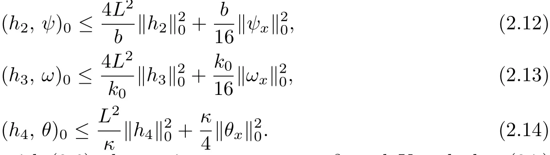
Then combining(2.8)–(2.14)with(2.6),there exist two constants β0and K such that(2.7)hold.The proof is completed.

2.2 Well-posedness

The existence of global mild and strong solutions to the thermoelastic Bresse system of type III will be established through nonlinear semigroup theory.We write the derivative ηsas an operator form,see,e.g.,[22].Define the operator T by

with

is the in finitesimal generator of a translation semigroup.In particular,

and the solution of

has an explicit representation formula.

Next we write the system(2.3)–(2.5)as an abstract Cauchy problem.Now we introduce four new dependent variables,then the system(2.3)–(2.5)is equivalent to the following problem for an abstract Cauchy problem.

where

and

with the domain

and

To obtain the solution of(2.15),we study the nature of the operator A+B.

Lemma 2.2 The operator A+B is maximal monotone in phase space H.

Proof.For all U∈D(A),by calculation,we have

then we can obtain the operator A is a dissipative operator.Now let

We prove the unique solution of the equation

Equivalently,we have the following system

From the last equation of(2.16)and η(0)=0,we infer that

By using(2.16)and(2.17)we can get the following problem

where

In the sequel,we define a bilinear form

given by

It is easy to verify that B is continuous and coercive.By using the Lax-Milgram theorem,the elliptic problem(2.18)has a unique weak solution(φ,ψ,ω,θ)∈ ((0,L))4.It is clear that η(x,0)=0 and ηs∈ M.To prove that η∈ M,let T,ϵ>0 be arbitrary.Using(1.14)and(1.15),we have

For(2.19)using η(x,0)=0,then as T → ∞ and ϵ→ 0,we obtain

It follows that

which gives us η∈ M.Therefore U(t)∈ D(A)solve the problem U −AU=U∗.

By using the same method as Theorem 2.2 in[4]and also in[23],we can prove the operator B is monotone,hemicontinuous and a bounded operator.

From above we know that the operator A+B is maximal monotone in H.The proof is thus completed.

Thanks to Lumer-Phillips theorem(see[24]),we deduce that A+B generates a semigroup of contractions in H.

Theorem 2.1(Well-posedness) Assume that(1.4)–(1.15)hold.Then for any initial data U0∈H and T>0,problem(2.15)has a unique mild solution

given by

and depends continuously on the initial data.In particular,if U0∈D(A),then the solution is strong.

Proof.Under Lemma 2.2 we have proved that A+B is maximal monotone in H.Then from standard theory the Cauchy problem

has a unique solution.We will show that system(2.15)is a locally Lipschitz perturbation of(2.21).Then from classical results in[25],we obtain a local solution define in an interval[0,tmax),where,if tmax<∞,then

To show that operator F:H→H is locally Lipschitz.Let G be a bounded set of H and U1,U2∈G,we can write

Then from assumption(1.5),we infer that for j=1,2,3,

and from assumption(1.9),we infer that

Then we infer that,for some CG>0,

Summing this estimate on j and f4we obtain

which shows that F is locally Lipschitz on H.

To see that the solution is global,that is,tmax=∞,let U(t)be a mild solution with initial data U0∈D(A+B).Then it is indeed a strong solution and so we can use energy inequality(2.7)to conclude that

By using density argument,this inequality holds for mild solutions.Then clearly(2.22)does hold and therefore,tmax=∞.Then the solution U(t)is a global solution.

Finally,by using(2.20)we can check the continuous dependence on initial data.Given T>0 and any t∈(0,T),we consider two mild solutions U1and U2with initial data U1(0)and U2(0),respectively.By(2.20),we get

which,using the local Lipshitz property of F and(2.7),give us

Then,applying the Gronwall’s inequality,we can obtain for any t∈ [0,T],

where

which shows that the continuous dependence on initial data.

By using Theorem 6.1.5 in[24],we can get that any mild solutions with initial data in D(A+B)are strong.

3 A Strict Lyapunov Functional

This section tries to find a strict Lyapunov functional to verify that(H,S(t))is a gradient system.It helps to obtain the existence and geometric structure of global attractor for(H,S(t)).

Define

where

Lemma 3.1 Φ is bounded from above on any bounded subset of H and the set ΦR={U(t):Φ(U(t))≤ R}is bounded for every R>0.

Proof. It is obvious

Then we can obtain t 7→ Φ(U(t))is non-increasing for every U0=(φ0,ψ0,ω0,θ0,φ1,ψ1,ω1,θ1,η0)∈ H with

It is obvious that Φ is bounded from above on bounded subsets of H.By(1.7)and the compact embedding frominto Lq1(q1≥1),there exist two constants>0,>0,such that

Combine with(2.7),we have

This is enough to show that ΦRis a bounded set of H.The proof is completed.

Lemma 3.2 Φ is a strict Lyapunov functional for dynamical system(H,S(t))on H.

Proof.Let

and

Then we have

which implies

and

By using the hypothesis(1.12),we can conclude from(3.2)that for any t≥0,

So,for all t≥0,

By using(3.3)and the condition(1.15),we know that for all t≥0,

Therefore,

follows from(2.2).

This gives us that

is stationary solution.The proof is completed.

Lemma 3.3 The set N of stationary points of(H,S(t))is bounded.

Proof. A stationary point U=(φ,ψ,ω,θ,0,0,0,0,0)∈ N of problem(2.3)satisfies the following equations:

Now multiplying(3.4)by φ,ψ,ω,θ,respectively,and integrating the resultant over(0,L),we have

By using(1.6)and F is a non-negative function,we can obtain

By(1.11),

Combining(2.9)–(2.14),we can infer that there exists a positive constant C such that

The proof of is completed.

4 Quasi-stability

In this section,we establish the quasi-stability of semigroup generated by global solution of problem(2.3)–(2.5).

Let B⊂H be a bounded positively invariant set of(H,S(t)),

be the two corresponding solutions with respect to initial data

We denote

and

with the Dirichlet boundary condition and the initial condition

Our objective is to obtain an estimate for E(t).

Lemma 4.1 For any ϵ1>0,there exists a positive constant CB(ϵ1)such that

Proof.We multiply equations(4.1)by,respectively,integrate the result over(0,L)and use the fifth equation of(4.1)to conclude that

(i)Forcing terms.

By using(1.5),H¨older’s inequality and Young’s inequality,we can get

Similarly,we have

By using(1.9),we have

(ii)Damping terms.

It follows from(1.13)that

Inserting(4.3)–(4.9)into(4.2),we obtain Lemma 4.1.

Let

Lemma 4.2 For any ϵ2>0,there exist constants c ≥ 0,C1(δ,ϵ2)>0,C2(ϵ2)>0 such that

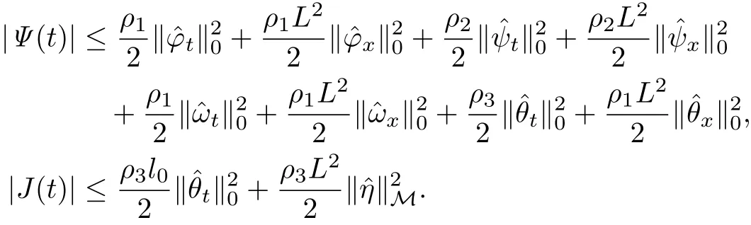
Proof. Taking the derivative of Ψ ,by using(4.1)and H¨older’s and Young’s inequalities,we can obtain

(i)Forcing terms.

By using H¨older’s and Young’s inequalities,we can get

and

By using(1.10),we can get

(ii)Damping terms.

Applying(1.13),we can obtain

and

Combining(4.11)–(4.17)with(4.10),we make the conclusion.

Let

Lemma 4.3 There exists a positive constant CBsuch that

Proof. Taking the derivative of J(t),we have

By using(2.2),we get

From the fourth equation of(4.1)and using H¨older’s and Young’s inequalities,we can obtain

It follows from Young’s inequality that

Combining(4.19)–(4.21)with(4.18),we make the conclusion.

Let

Then we can obtain the following Lemma.

Lemma 4.4 The dynamical system(H,S(t))is quasi-stable on any bounded positively invariant set B⊂H.

Proof.Using Young’s inequality and Poincar´e’s inequality we can know

Thus there exists a constant β0′>0 such that

Take the derivative of L(t)and combing with Lemmas 4.1–4.3,we can obtain

We choose ε1,ε2,ϵ1,ϵ2enough small such that

Then,combine with(4.23),we conclude that there exists a constant r0>0 and a constant CB>0,depending on B,such that

By using(4.22),we have

If we use(4.22)again,we can obtain

Since the system(H,S(t))is defined as the solution operator of problem(2.15),we conclude that Assumption 7.9.1 of[10]hold with X=((0,L))4,Y=(L2(0,L))4×M.Moreover,from the continuous dependence on initial date,we can obtain

By the compact embedding theorem,

where

It is easy to get that

Since B ⊂H is bounded,we know that c(t)is locally bounded on[0,∞).Therefore the Definition 7.9.2 of[10]hold,that is,the dynamics system(H,S(t))is quasi-stable on any bounded positively invariant set B⊂H.The proof is hence completed.

5 Global Attractor and Exponential Attractor

In this section,we prove the existence of attractor which has finite fractal dimension and the exponential attractors of the system is also existed.

Theorem 5.1 Assume that the hypotheses(1.4)–(1.15)hold.Then the dynamical system(H,S(t))generated by the problem(2.3)–(2.5)has a compact global attractor A which is characterized by

where N is the set of stationary points of S(t)and M+(N)is the unstable manifold emanating from N.

Proof.By Lemma 4.4 and Proposition 7.9.4 of[10],the dynamical system(H,S(t))is asymptotically smooth.By Lemma 3.1–3.3,we make the result from Corollary 7.5.7 of[10].

The following theorem investigate the finite dimensionality and regularity on time of the attractor A.

Theorem 5.2 The attractor A has a finite fractal dimensionFurthermore,any full trajectory{(φ(t),ψ(t),ω(t),θ(t),φt(t),ψt(t),ωt(t),θt(t),η(t)):t∈ R}in A has following regularity

Moreover,there exists an R>0 such that

where R>0 depends on the attractor A.

Proof.From Theorem 5.1 and Lemma 4.4,we obtain the results by using Theorem 7.9.8 of[10].

Under Definition 7.9.2 of[10],we easily obtain the result on the existence of generalized exponential attractor.

Define

where η′is the weak derivative of η.Its inner product is

We obtain the existence of generalized exponential attractor in H for the dynamical system(H,S(t)).

Theorem 5.3 Assume that(1.4)–(1.15)hold.Then the dynamical system(H,S(t))possesses a generalized exponential attractor Aexp⊂H,with finite fractal dimension in extended space

Proof.Now we take

where Φ is the strict Lyapunov functional considered in Lemma 3.1.Then we know that the set B is a positively invariant absorbing set for R large enough.Hence the system(H,S(t))is quasi-stable on B.

For the solution U(t)with initial date y=U(0)∈B,since B is positively invariant,