Adaptive optimization methodology based on Kriging modeling and a trust region method

Chunna LI,Qifeng PAN

aInstitute of Space Planes and Hypersonic Technologies,School of Astronautics,Northwestern Polytechnical University,Xi'an 710072,China

bFaculty of Aerospace Engineering and Geodesy,University of Stuttgart,Stuttgart 70174,Germany

Abstract Surrogate-Based Optimization(SBO)is becoming increasingly popular since it can remarkably reduce the computational cost for design optimizations based on high- fidelity and expensive numerical analyses.However,for complicated optimization problems with a large design space,many design variables,and strong nonlinearity,SBO converges slowly and shows imperfection in local exploitation.This paper proposes a trust region method within the framework of an SBO process based on the Kriging model.In each refinement cycle,new samples are selected by a certain design of experiment method within a variable design space,which is sequentially updated by the trust region method.A multi-dimensional trust-region radius is proposed to improve the adaptability of the developed methodology.Further,the scale factor and the limit factor of the trust region are studied to evaluate their effects on the optimization process.Thereafter,different SBO methods using error-based exploration,prediction-based exploitation,refinement based on the expected improvement function,a hybrid refinement strategy,and the developed trust-region based refinement are utilized in four analytical tests.Further,the developed optimization methodology is employed in the drag minimization of an RAE2822 airfoil.Results indicate that it has better robustness and local exploitation capability in comparison with those of other SBO methods.

KEYWORDS Airfoil;Design optimization;Kriging model;Surrogate-based optimization;Trust-region method

1.Introduction

In modern optimization design of flight vehicles,many complicated and time-consuming numerical analysis techniques,such as Computational Fluid Dynamics(CFD)and Computational Structural Mechanics(CSM),have been employed.1-6Many design variables and complex couplings bring more difficulty to the optimization process,especially for Multidisciplinary Design Optimization (MDO).7-10Although the adjoint method11has been applied to improve the optimization efficiency,the method is still limited to local optimization problems.12Surrogate model provides an alternative to handle complicated optimization problems with many design variables and multiple optima,and has sparked much interest in MDO.13-15

The optimization process,exploring the design space based on a surrogate model,is called Surrogate-Based Optimization(SBO).Within the process,the surrogate model is used to replace expensive numerical analyses or experimental measurements in a conventional optimization process.16There are many different surrogate models,such as the polynomial Response Surface Model(RSM),17the Kriging model,18Radial-Basis Functions(RBFs),19Support-Vector Regression(SVR),20and Neural Network(NN).21Among them,the Kriging model developed by Krige in 195218is a representative modeling method,which is suitable for nonlinear problems.Besides,the Kriging model can provide approximations of an unknown function as well as their error estimations,which is beneficial for SBO.

In SBO using Kriging modeling,another important technique is the refinement strategy,because it has a great influence on the efficiency,robustness,and quality of the optimization process.After building an initial surrogate model,new samples carrying more information of the optima and the design space should be added into the database in each refinement cycle(iteration).The refinement strategy relates to the rules or methods of selecting those new samples.22At present,there are five commonly used refinement strategies:23,24prediction-based exploitation,error-based exploration,Expected Improvement(EI)-based refinement,refinement based on the Probability of Improvement(PI),and a statistically lower confidence bound.In abovementioned strategies,EI-based refinement can always balance local exploitation and global exploration.

Currently,more efficient refinement strategies are being of concern.Ginsbourger et al.developed aq-EI-based refinement strategy25by selecting a number ofqsamples in each refinement cycle and employing parallelization to search faster.A hybrid refinement strategy,26,27which generates multiple new sample points in one refinement cycle,can get better performance in handling complicated optimization problems with many design variables and multiple optima.However,for optimization problems with a large design space,many design variables,and strong nonlinearity,the adaptability of a refinement procedure using the above strategies is insufficient,especially with an initial sampling plan lacking enough information of the design space.28A sampling criterion for RBF-based interpolation has been developed by Mackman et al.using a response surface curvature and a sample separation function,to achieve two aims:local refinement and exploration of the domain.29Chaudhuri et al.combined PI-based refinement with a trust region method,which is named as Efficient Global Optimization with Adaptive Target(EGO-AT),to search more adaptively.30Long et al.proposed to use a trust region method in SBO using an RBF model,to guarantee a dynamic adaptive search.31

Besides,variable- fidelity surrogate modeling and Gradient-Enhanced Kriging(GEK)can be used in improving the efficiency of refinement and the local model accuracy.Han and Görtz proposed a hierarchical Kriging model for variable fidelity surrogate modeling problems,in which the model trend is coordinated by a model built by lower- fidelity data.32Koziel and Leifsson used a low- fidelity model and data obtained from one high- fidelity model evaluation in each design iteration for building a surrogate model.33Cokriging was initially proposed for an enhanced prediction of less intensive samples by means of auxiliary variables.34Han et al.proposed an alternative approach for the construction of a cokriging covariance matrix and developed a more practical cokriging method.35GEK is viewed as one kind of cokriging,in which cheap gradients are incorporated to enhance the local model accuracy.A newly developed generalized hybrid bridge function has been combined with direct GEK in order to improve the efficiency and accuracy of variable- fidelity surrogate modeling.36Recently,a novel weighted GEK has been proposed in combination with cheap gradients by an adjoint method especially for high-dimensional problems.37

In this work,we propose an efficient adaptive sampling based on the trust region(TR)method to improve the convergence of an SBO process based on the Kriging model.Since it is also a type of SBO,we dub the methodology SBO-TR.Factors for controlling the update of the trust region are studied,aiming to appropriately set the developed optimization methodology.Similar to a hybrid refinement strategy,SBOTR can also take advantage of parallelization of computing new samples per refinement cycle,in order to further improve searching efficiency.

2.Methodology

2.1.Kriging modeling

The Kriging model was originally proposed in 1951 by Krige,18a geologist from South Africa,to interpolate an unobserved value in a random field by using observations nearby.In the 1970,38a French mathematician,Georges Matheron,developed a regional-variable theory and coined it Kriging.Sacks et al.39applied Kriging modeling in deterministic computer simulations for the first time in 1989.

Suppose that we are handling anm-dimensional problem,and we want to build a Kriging model for an unknown functiony:Rm→R with respect to design variables x.The unknown function could be the objective function or a constraint function,which is expensive to evaluate.Thus,an initial sampling plan within the design space is needed by a certain Design of Experiment(DoE)method.The sampled data set isBy high- fidelity analyses(could be CFD or CSM)ofnsamples,the functional responses could be obtained asThe sampled data and the computed corresponding responses are then used for building the Kriging model.

The Kriging model is an interpolating model based on the statistics theory,which can be expressed as follows:

where x is the vector with all the design variables,and^Y（ x）is the predicted function value at a certain x by interpolating the Kriging model;μ is the regression parameter denoting the mean of the observations used for building the model;Z(x)represents a stochastic process with a zero mean.AsZ(x)shows a local deviation from the model,it can be calculated by evaluating the correlation between the local position and the nearby observations.The covariance matrix ofZ(x)can be calculated using the correlation matrix as

where R is the correlation matrix,and σCis its variance.In the above formula,the elements of R can be computed by

whereR(xi,xj)is the Gaussian correlation function between samples xiand xj;nis the number of samples;θlis thelth(l∈ ［1，m］)unknown correlation parameter40for tuning the surrogate model,whereinmis the number of design variables.This function controls the influence on the local model accuracy by neighbouring samples as well as the smoothness of the model.Thus,the resulting Kriging model can be expressed as

In order to evaluate θ,the concentrated logarithm likelihood function shown in Eq.(6)should be maximized by running optimization algorithms.Generally,there is no limitation on such optimization algorithms,but only considering their efficiency.

Then the mean square error of the Kriging model can be expressed by

2.2.Trust region method

The TR method was firstly used to solve unconstrained optimization problems by Powell,41of which the distance between the iteration points in the current iteration cycle and the cycle before should be limited.In the method,a quadratic model by Taylor-series expansion is used to approximate the objective function.It can be thought that there is a neighborhood around the current iteration point,within which we trust the surrogate model.Such a neighborhood is called a trust region.The size of the trust region is tuned by the performance of the algorithm in previous search.42If the model is generally reliable,being able to generate a good search step and accurately predict objectives,the size of the trust region can be increased.In reverse,a bad search step indicates that the model is inadequate in representing the objective function within the trust region,and thus the size of the trust region needs to be reduced.

The unconstrained optimization problem can be normally expressed by

whereNmrepresents anm-dimensional design space.

The quadratic model centered at the current iteration point xkby Taylor-series expansion is

where the gradient vector is gk= ▽f（ xk）,and the Hessian matrix is Hk= ▽2f（ xk）22.Within the trust region around the current iteration point xk,the search step Δx should be specified by solving the following optimization problem:

wherehkstands for the upper bound of the search step Δx in thekth iteration cycle.A suitablehkcan guarantee that the series containing iteration points{xk}converges to x*.To obtainhk,a trust factor λ is introduced in describing the similarity between the quadratic modelq(Δxk)and the objective functionf(xk+ Δxk).Suppose that Δfk=f(xk)-f(xk+ Δxk)is the actual reduction of the objective function in thekth iteration cycle,and Δqk=f(xk)-q(Δxk)is the predicted reduction of the objective function.Thus,the trust factor is defined by

As the search step Δx is limited by minimizing the model in Eq.(10)over a neighborhood including Δx=0,the predicted reduction is always nonnegative.If λkis negative,the search step is not good,and should be rejected;while if λkis close to 1,the quadratic modelqkagrees quite well with the actual objective function within the trust region,and thus the trust region can be expanded in next iteration cycle,which means thathkshould be amplified.

We apply the trust region method into an SBO to tune the design space for selecting new samples.The size of the trust region changes according to the accuracy of the surrogate model,and thus new samples selected within the trust region can further improve the model accuracy locally.The variable design space can guide the search to the global optimum adaptively.

2.3.Adaptive optimization process

2.3.1.Surrogate-based optimization

A general nonlinear optimization problem withmdesign variables can be expressed as

wheregj(x)are constraints;are the lower and upper bounds of theith design variablexi,respectively.

In an SBO,an initial set of samples need to be firstly generated by a certain DoE method to describe the design space.There are a number of conventional and modern DoE methods,24such as the full factorial,the central composite,the D-optimal,the stratified Monte Carlo,the Latin hypercube,and the orthogonal array methods.Different sampling plans have different model accuracies,which will affect the efficiency of an SBO.For a basic SBO process,the initial surrogate model should possess a good enough model accuracy.According to Ref.22 the quantity of initial samples generated by DoE should be larger thanm(m+1)/2.In our work,the Random Latin Hypercube Sampling(RLHS)and its variant that can generate more uniform distributed sampling plans are available in the SBO process.28Then high- fidelity analyses are carried out to obtain observations for those samples.

Thereafter,the refinement procedure of most importance starts,within which different refinement strategies can be applied to obtain new samples in each iteration cycle.In the work,the hybrid refinement strategy26and commonly used refinement strategies,including prediction-based exploitation,error-based exploration,and EI-based refinement,are available.Then high- fidelity analyses of the new samples are carried out to expand the database in order to update the model accuracy.

The refinement procedure will stop when the criteria estimating the model accuracy are satisfied.Finally,the surrogate model can be used to predict objectives in the optimization in lieu of a high- fidelity analysis tool,or the current best sample in the database is taken as the optimum.Details of the flow chart for the basic SBO process can be seen in Fig.1.

Adaptive optimization is an iterative procedure.Hence,criteria are needed to terminate this iteration.To guarantee a globally-correct and locally-accurate surrogate model within a limited quantity of observations,multiple criteria are needed.In the developed optimization procedure,the following convergence criteria are employed.

(1)A threshold for the objective function:in case that the current best objective goes beneath this threshold,the refinement stops.The criterion is on the premise of a known target objective value.

(2)Two tolerances for sequential best observations:if the discrepancy between the updated best observation and the previous best observation goes below a certain small tolerance,as well as the maximum distance in a certain dimension between the two locations of those two observations is smaller than a tolerance,the refinement stops.

Fig.1 Flow chart of basic SBO.

(3)The tolerance for the maximum Kriging error:as Kriging modeling is used to search for the local optimum,when the maximum Kriging error is zero or smaller than a defined tolerance,the refinement can be terminated.

(4)The maximum of the cumulated step within which the best observation has no update:when the cumulated step is larger than the pre-defined maximum,the refinement stops.

(5)The limitation of the maximum refinement cycles:when the refinement procedure has run beyond the limitation,the refinement stops.This criterion is always regarded as the most general criterion for the refinement procedure,which is always defined with surplus

2.3.2.Sampling with a variable design space

Since the trust region can be adaptively updated by considering the performance of previous search,42we introduce the trust region method into the basic SBO process to adjust the design space for sampling,aiming to obtain an adaptive optimization process.We dub the methodology SBO-TR,as is shown in Fig.2.To update the trust region,three essential factors should be identified firstly:the trust factor,the trustregion center,and the trust-region radius.

Based on Eq.(11),we can compute the trust factor by

The trust-region center is defined as the location of the optimum on the surrogate model.During the refinement procedure,the optimum on the surrogate model in the current iteration cycle is compared with the one in the previous cycle,to decide whether to update the trust-region center:ifkeep the original trust-region center;if

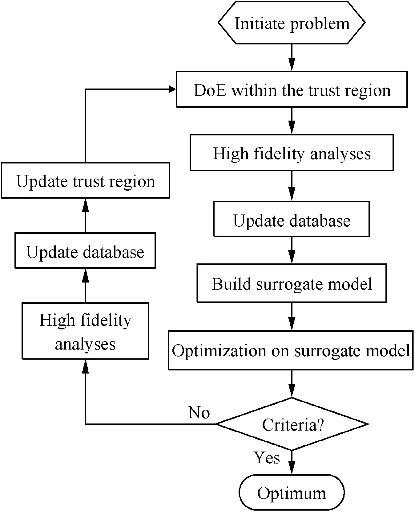
Fig.2 Flow chart of SBO-TR.

update the trust-region center by xc=

Knowing the trust-region center,the design space for selecting new samples can be encompassed by the trust-region radius around the trust-region center.In the conventional trust region method,the trust region is a generalized hypersphere,31and thus the trust-region radius ρ is a value.In our work,considering the sensitivity of each design variable to the objective function,we suppose that the trust region is a hypercube.Hence the developed methodology has a multiple dimensional trust-region radius ρ,which is a vector withmelements.Such a treatment is in favor of efficiency of the refinement procedure,especially for problems sensitive to partial design variables.

To compute the trust-region radius,we need to firstly identify the scale factor of the trust region by

wherec1,c2,r1,andr2are specified parameters,which are generally defined asc1=0.75,c2=1.25,r1=0.1,andr2=0.75;λkis the trust factor of thekth refinement cycle;κkis the scale factor of thekth refinement cycle.If λk＜r1,indicating that the local accuracy of the current model is not good,the radius of the trust region should be shrunk byc1;if λk＞r2,showing that the model is locally accurate enough,the trust-region radius will be amplified byc2,;ifr1≤λk≤r2,it means that the current local model accuracy needs to be improved,and hence the trust-region radius remains unchanged,as is shown in Fig.3.

Hence,the elements of the multiple-dimensional trustregion radius ρkin thekth refinement cycle can be computed by

To suppress being fast trapped into a local optimum,a limitation to the trust-region radius vector should be added.Thus,the multiple-dimensional trust-region radius could be revised by

where γ is the limit factor,and ρ0is the initial trust-region radius vector.The common setting of the limit factor is 0.05.Then the lower and upper bounds of the trust region in thekth refinement cycle can be computed using

SBO-TR is detailed as follows:

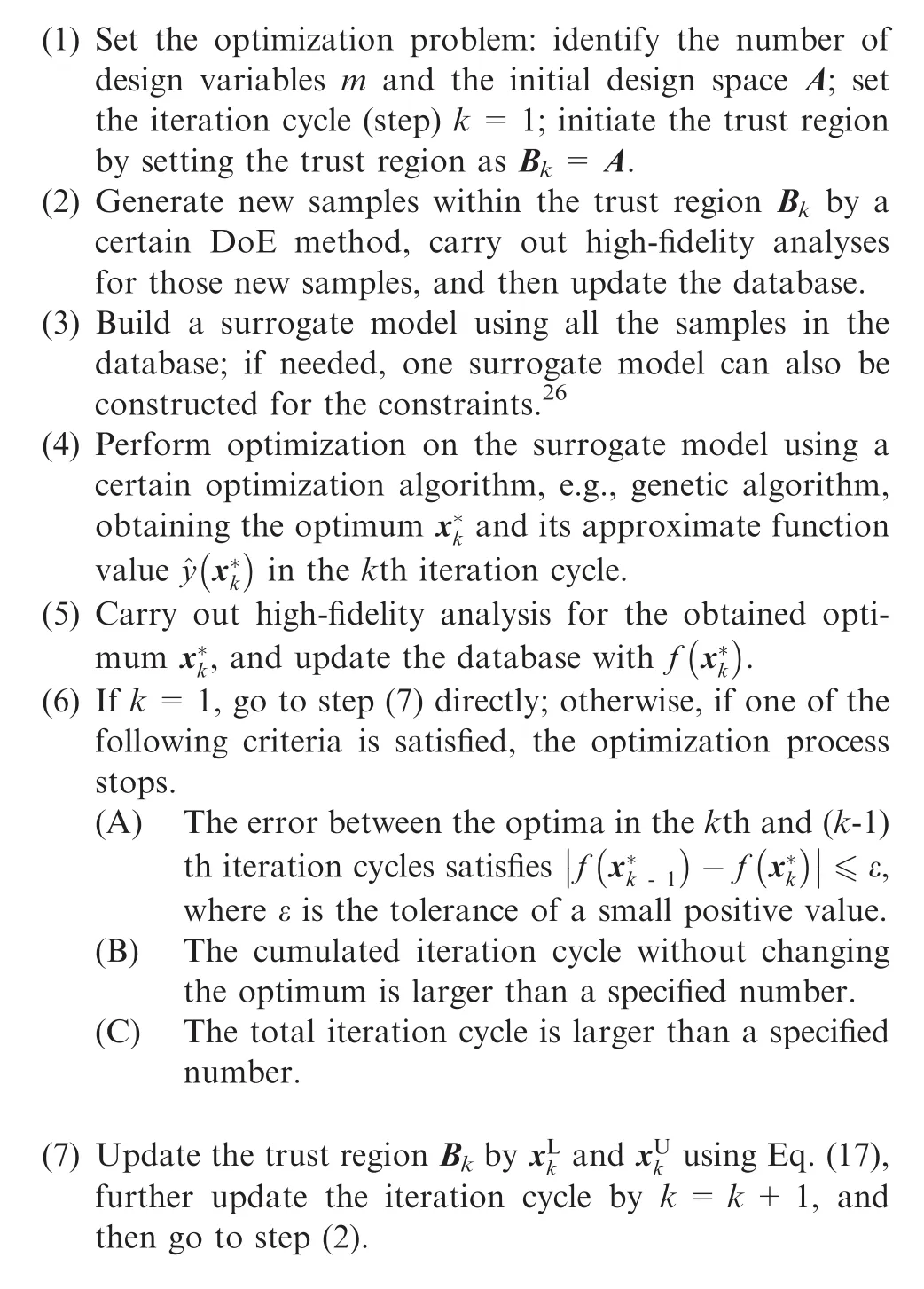
Fig.3 Illustration of updating the trust region(no limitation by the minimum size of the trust region,and the updated trust region also does not exceed the design space).

2.3.3.Study of factors in trust-region method

Theoretically,the scale factor decides the size of the updated trust region.If it is too small,as the number of new samples added into the database is the same in each refinement cycle,the local region of the design space can be delicately described with intensive samples.Besides,a small-scale factor tends to be easily trapped into a local optimum.In reverse,a large-scale factor will result in many redundant samples,which will reduce local model accuracy.Hence,we need to appropriately set the scale factor to control the refinement procedure.In view of Eq.(14),the scale factor is decided by parametersc1andc2.

The 2D Rosenbrock function,with a global optimum of 0 located at(1.0,1.0),is utilized to study the effect of the scale factor on SBO-TR.Since the function has a narrow long ridge,it is difficult in generating a good search direction by global optimization algorithms,as is shown in Fig.4.The optimization problem can be expressed as

A test has been carried out by setting 16 combinations ofc1andc2,as is shown in Table 1.For each set ofc1andc2,the optimization has been run ten times to examine the robustness of the methodology.The optimum,the number of samples,and the variance are all average values of the ten runs.The variance is computed by

whereis the optimum for theith optimization out of the ten runs;is the expected optima for all the runs if there is no analytical optimum,or else is the analytical optimum.Thus,the variance represents the robustness of the optimization process.

Generally,with a fixedc1,increasingc2can result in a smaller optimum and variance.It indicates that a smallerc2is good for optimization quality and robustness,but at expense of calculating the objective function more times.With a specifiedc2,increasingc1can lead to a ‘down-up-down” trend for the optima.However,the change of such a trend becomes much smaller along with increasingc2.In fact,a largec2is not recommended,because it will cause too many samples in the database,which can slow down the optimization process and take more time in building surrogate models.In view of many testcases,c1=0.75 andc2=1.25 are recommended for common problems,whilec1=0.55 andc2=2.00 for strong nonlinear problems.

Fig.4 Zoomed-in contour of the 2D Rosenbrock function.

After a number of iterations for the refinement,the trustregion radius might become very small,which could make the optimization trapped into a local optimum for problems with strong nonlinearity or result in difficulty in further improving local model accuracy.31We introduce a limit factor γ for the trust-region radius to tune the refinement procedure,as is seen in Eq.(16).The effect of the limit factor is also studied using the 2D Rosenbrock function withc1=0.75 andc2=1.25,and results are shown in Table 2.

Theoretically,a smaller limit factor is in favor of better optimization quality and robustness,but it will take a higher computational cost.However,a too small limit factor can cause more numerical noise in the local region for building surrogate models,which might lead to a bad optimum or even failure in building models.In view of the results in Table 2,a limit factor of 0.05 is recommended.

3.Test cases

3.1.2D analytical test cases

The Six-hump Camel back(SC)function is a standard test case with multiple optima,and the 2D Griewank(GN)function has strong nonlinearity due to great many optima.Thus,the two functions are utilized to validate and assess the developed methodology.The SC function has six optima,as is shown in Fig.5(a).Two of the optima,both-1.0316,are global,which are located at(0.089842,-0.712656)and(-0.089842,0.712656),respectively.The optimization problem is written as

The GN function has one global optimum of many optima,as is shown in Fig.6(a).The global optimum is 0 located at(0,0).The nonlinearity of this function is very strong.When the design space is large,the search will easily fall into a local optimum.The optimization problem is described by

For each test case,the global-search Difference Evolution(DE)43algorithm,and SBOs using prediction-based exploitation(SBO-MSP),24error-based exploration(SBO-KE),EI-based refinement(SBO-EI),hybrid refinement(SBO-Hybrid),and the trust region method(SBO-TR),are performed.For all the tests using SBO,only four initial samples are generated by the RLHS,guaranteeing at least two samples in the projection along each design dimension.Thus,an initial surrogate model can be built by the four samples plus the baseline sample.In SBO-MSP,the optimum on the surrogate model is selected as an in fill sample in each refinement cycle;in SBOKE,the location of the maximum model error is selected to add an in fill sample in each refinement cycle;in SBO-EI,the location with the maximum expected improvement function value is chosen to add an in fill sample in each refinement cycle.In comparison,totally three samples including one from prediction-based exploitation,one from error-based exploration,and one from EI-based refinement are selected as in fill samples in each refinement cycle in SBO-Hybrid.In SBO-TR,five samples are generated by the RLHS and added into the database in each refinement cycle.The parameters for SBOTR are set as follows:γ=0.05,c1=0.75,c2=1.25,r1=0.1,andr2=0.75.

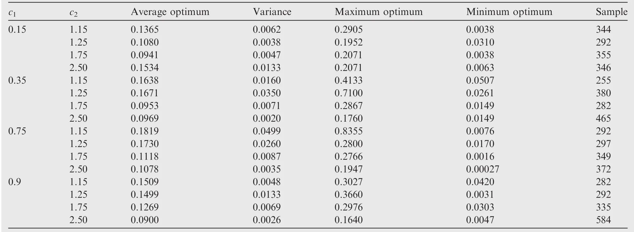
Table 1 Effects of c1and c2on SBO-TR.

Table 2 Effect of the limit factor γ on SBO-TR.

Each test by SBO has been repeatedly performed ten times by the same optimization methodology to evaluate the robustness of the method.Hence,the optimum from each methodology is the average optimum of ten runs,and the number of samples is also the average value.The optimization results of the two 2D tests are detailed in Tables 3 and 4,respectively.To distinguish the maximum and minimum optima for the optimization of the SC function,we take six digits after the decimal point.

The DE algorithm can always find the global optimum at expense of calculating the function thousands of times.The SBO methodology depends greatly on the refinement procedure.A good refinement procedure can guarantee an efficient selection of in fill samples with a good distribution,which signifies a correct landscape of the global design space and an accurate description of the local region around the optima.

Out of the ten runs by each SBO method,the best case is selected to be compared.The samples in the database for each SBO method are finally displayed in Figs.5 and 6,and the contours depicted by the samples are also compared as well.It can be seen that SBO-EI,SBO-Hybrid,and SBO-KE are global methods,because they can find almost all the optima in the design space.In comparison,SBO-KE is incapable in local exploitation due to sparse samples in the local regions,as is shown in Figs.5(f)and 6(f),while SBO-EI shows drawbacks in global exploration in view of the contours in Fig.5(b).SBO-MSP and SBO-TR are essentially local methods with respect to their sample distributions.However,SBO-TR will not be fast trapped into a local optimum nearby(Figs.5(d)and 6(d)),due to uniformly selecting in fill samples within trust regions,of which the initial trust region is the complete design space.In comparison,SBO-MSP will directly focus on the optimum in the neighborhood,which can be seen in Figs.5(e)and 6(e).

In view of Figs.7 and 8,SBO-TR has the best robustness,because the optima(black diamonds)obtained are mostly concentrated around the theoretical optima.SBO-MSP has difficulty in handling problems with strong nonlinearity,as the ten optima(red squares)obtained are dispersedly distributed.Although SBO-KE shows concentrated optima(pink circles)for the SC test case,but it is resulted from the local low accuracy of the surrogate model.It indicates that SBO-KE is incapable in local exploitation.In comparison,SBO-EI and SBO-Hybrid can take all optima into account,but show incompetence in local exploitation for highly-nonlinear problems.

The ten optima by each SBO method are compared in Figs.9 and 10.It indicates that,for problems with a low dimensional design space and weak nonlinearity,all the SBOs have good robustness.However,for problems with strong nonlinearity,their robustness all decrease,among which SBO-KE has the worst robustness while SBO-TR behaves best.Thus,SBO-TR possesses the best optimization quantity and robustness.

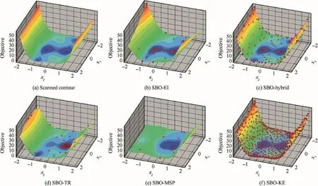
Fig.5 Comparison of contours and sample distributions between SBOs with different refinement strategies for the SC function(the best case out of ten runs).

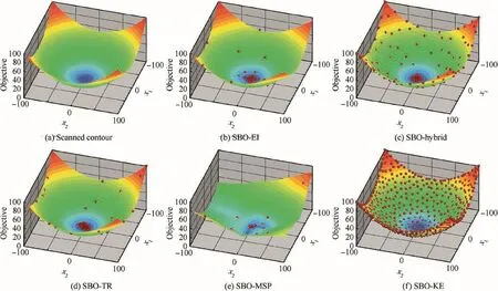
Fig.6 Comparison of contours and sample distributions between SBOs with different refinement strategies for the GN function(the best case out of ten runs).

We take the optimization obtaining the best optimum out of the ten runs by each SBO method,to compare the convergence feature of the developed methodology.The convergence

histories of the refinement procedure are compared in Fig.11 for the SC and GN functions.Since the extension of the objectives for the GN function is large,we take the logarithm of the objective as the vertical axis.For optimization problems with weak nonlinearity,e.g.,the SC function,the convergence feature has no big difference for all the SBO methods except SBO-KE,which shows incompetence in local exploitation.However,SBO-TR converges a litter faster than the others.For problems with strong nonlinearity,such as the GN function,generally SBO-TR shows the best convergence feature.The reason why SBO-MSP obtains a better optimum in current circumstance is that the result is the best one out of the ten runs,which is not the typical case.It can also be explained by the robustness analysis of SBO-MSP shown in Table 4.Likewise,SBO-KE also shows the worst performance in local exploitation.

Table 3 Results of optimizing the SC function.

Table 4 Results of optimizing the GN function.

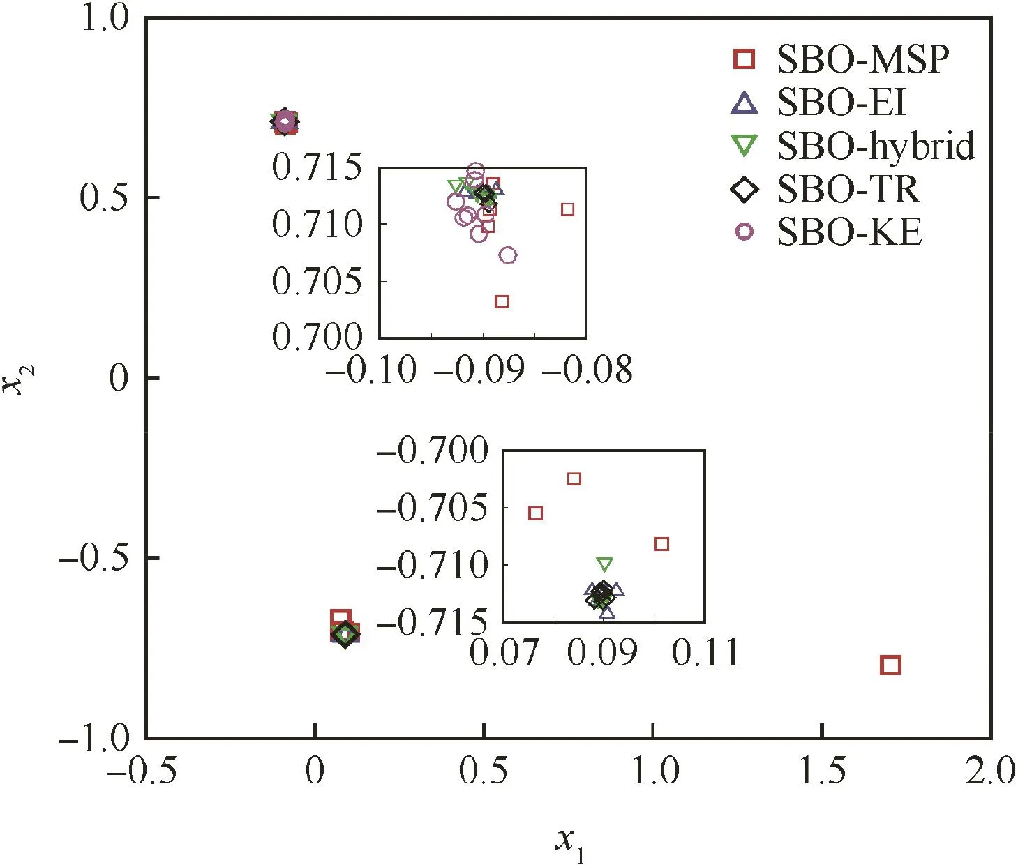
Fig.7 Optima of the SC function obtained by SBOs.

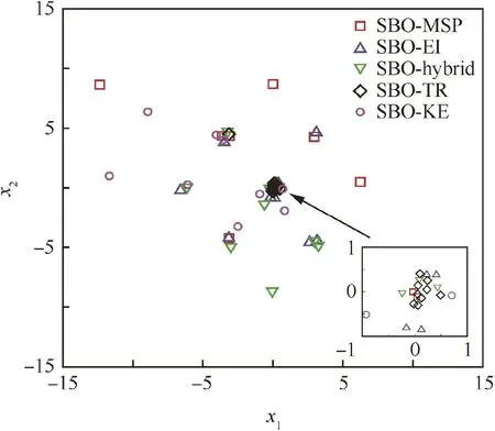
Fig.8 Optima of the GN function obtained by SB Os.

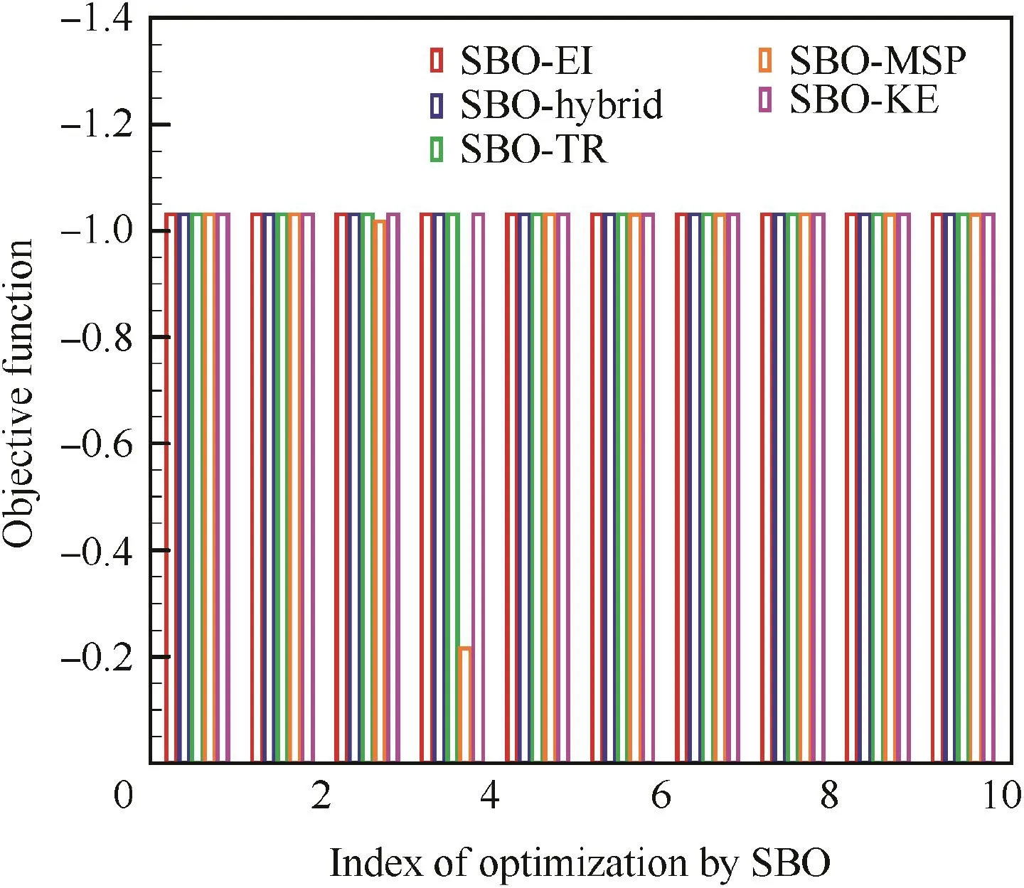
Fig.9 Optima comparison of the SC function for ten runs.

Fig.10 Optima comparison of the GN function for ten runs.

The objectives for all the samples of the SC and GN functions are compared in Fig.12.It is shown that SBO-KE and SBO-Hybrid are better at describing the objective function globally,because the objectives of the in fill samples are located within a large extension.SBO-MSP and SBO-TR focus on the local region and show a better local exploitation performance due to a narrow extension.In comparison,the samples chosen by SBO-EI can generally balance between global exploration and local exploitation.

Fig.11 Comparison of convergence histories of the refinement procedure for the SC and GN functions.

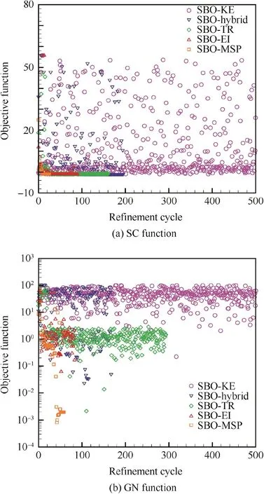
Fig.12 Comparison of objectives for all samples in the databases of the SC and GN functions.

3.2.Multiple-dimensional test cases

Two standard analytical test cases are performed to assess the developed methodology in handling high-dimensional problems:the 10D Rosenbrock(RB10)function and the HD1 function.31The two functions are typical high-dimensional tests.The RB10 function is difficult in identifying an appropriate searching direction because of the long ridge,while the HD1 function has strong nonlinearity.Both of the two optimization problems have a global optimum of 0,and they can be respectively expressed as follows:

Because SBO-MSP only focuses on local exploitation and SBO-KE is incompetent in local exploitation,only SBO-EI,SBO-Hybrid,and SBO-TR are utilized for high-dimensional test cases.Each SBO method has also been repeatedly executed ten times.The initial sampling plan includes 20 samples generated by the RLHS and the baseline sample,which can also guarantee at least two samples in the projection along each design dimension.The parameters in SBO-TR for optimizing the RB10 function are set as γ=0.05,c1=0.65,c2=2.0,r1=0.1,andr2=0.75,with respect to optimization quality.The parameters in SBO-TR for optimizing the HD1 function are:γ=0.05,c1=0.75,c2=1.25,r1=0.1,andr2=0.75.In each iteration cycle,six new samples are generated by the RLHS and added into the database.To assess the developed methodology,the DE algorithm is also performed with a setting of 40 populations and 200 generations.Results are compared in Tables 5 and 6.

Although the DE algorithm has computed the functions thousands of times,it still fails in finding a good global optimum for both tests.Normally,if we modify the settings in DE,e.g.,increase the population in each generation,a better optimum should be obtained at expense of calculating the function tens of thousands of times.

SBO-EI and SBO-Hybrid behave even worse in optimization quality as well as robustness.The reason might be that both of SBO-EI and SBO-Hybrid depend greatly on the initial sampling plan,especially for problems with a high dimensional design space.We have reset the initial sampling plan to 100 by the RLHS.For the test of optimizing the RB10 function,both SBO-EI and SBO-Hybrid have obtained better optima of 15.150 and 43.47,respectively.The average variances obtained are respectively 74.278 and 13.317,which are also much better.

SBO-TR behaves best,as the optima found are respectively 0.45387 and 0.04214,which are closest to the theoretical optima for both tests.In comparison with results by SBO using radial basis functions in Ref.31which are respectively 5.1690 and 0.5387,the optimization quality by the developed SBOTR is much better.However,considering the cost of computing functions,SBO-TR has performed 1072.00 and 1015.30 function evaluations,respectively,which are also more than 444.7 and 312.7 in Ref.31.The results are further checked in the log file from running SBO.It states that SBO-TR has found a transient optimum of 5.04087 in the iteration cycle of 46 with 343 function evaluations in optimizing the RB10 function,while a transient optimum of 0.41234 in the refinement cycle of 30 with 238 function computations in optimizing the HD1 function.It indicates that SBO-TR by using Kriging possesses better adaptability.

The ten optima obtained by SBO-TR have the smallest variance among the three SBO methods.It demonstrates that SBO-TR has the best robustness among the three SBO methods,which can also be drawn from Figs.13 and 14.

Fig.15 compares the convergence histories of the refinement procedure for optimizing the RB10 and HD1 functions.We also take the logarithm of the objective as the vertical axis since extensions of the objectives for both functions are large.It shows clearly that SBO-TR converges much faster than SBO-EI and SBO-Hybrid.Besides,SBO-TR has a much better convergence.

Fig.16 compares the objectives of all the samples by SBO methods for optimizing the RB10 and HD1 functions.SBOTR also exhibits a good capability in accurately describing the local design space.However,too many samples selected by SBO-TR need a higher computational cost.To avoid too many numerical simulations while providing a good enough optimization quality,suitable criteria for the refinement and the optimization process should be set.

In SBO-TR,the number of in fill samples defined within the trust region are dependent on the complexity of the objective function.There are no accurate criteria for the setting.However,in view of many tests,4-6 in fill samples are recommended for 2D problems,and 6-10 in fill samples are recommended for high-dimensional tests.When in fill samples are more than 10,the samples are over-accumulated within a small trust region after a certain number of refinement cycles,so the accuracy of the surrogate model reversely decreases.

Table 5 Results of optimizing the RB10 function.

Table 6 Results of optimizing the HD1 function.

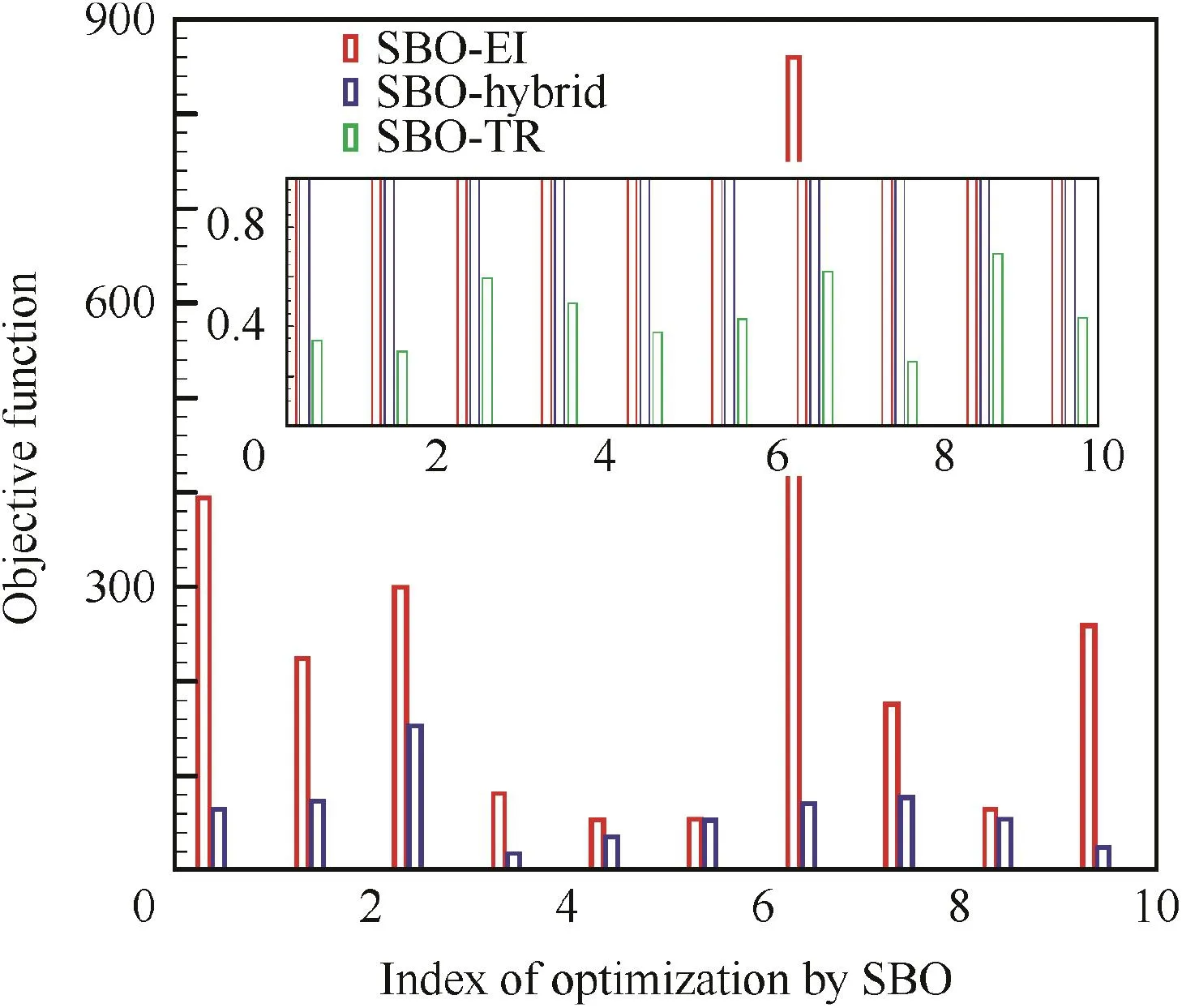
Fig.13 Optima comparison of the RB10 function for ten runs.

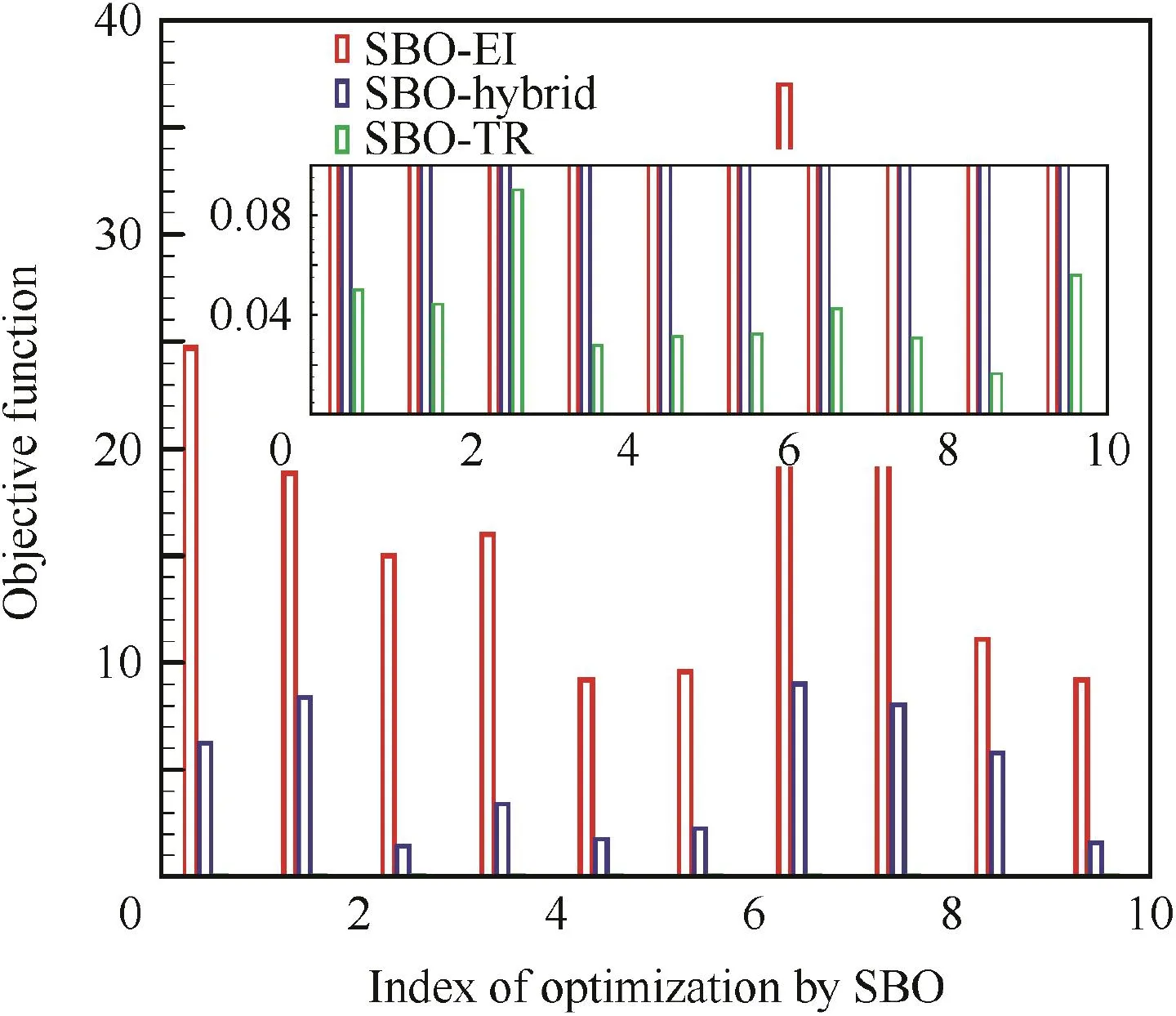
Fig.14 Optima comparison of the HD1 function for ten runs.

3.3.Optimization of an RAE2822 airfoil to reduce its drag

To validate the developed methodology in engineering applications,an RAE2822 airfoil is optimized to reduce its drag.The design point is α =2.31°,Ma=0.729,andRe=6.4 × 106.The optimization problem can be expressed as

whereCDandCLare the drag and the lift coefficient,respectively.

The geometry of the airfoil is discretized by the Hicks-Henne method with 38 control points,as is shown in Fig.17.The non-dimensional length of the airfoil is 1.Thex-coordinates of those control points are fixed,and the variations of they-coordinates of those control points are set as design variables.A hybrid mesh is generated by the commercial software Pointwise,and the mesh contains 22,842 mesh elements,as is shown in Fig.18.In the boundary layer,the height of the first layer is 1×10-5.

Fig.15 Comparison of convergence histories of the refinement procedure for the RB10 and HD1 functions.

Another fine mesh as well as a coarse mesh is generated by Pointwise to perform a grid convergence study.Both of the meshes have the same first-layer height as that of the medium,while the elements for them are respectively 13285 and 52237.Then CFD computations at the design point are carried out for all three meshes using the open-source CFD code SU2.The lift and drag coefficients are compared in Table 7.It shows that the lift and drag coefficients by using the medium and the fine meshes converge to a constant value.Thus,the medium mesh used in optimization meets the convergence condition.Besides,the pressure-coefficient curve by using the medium mesh is compared with experimental data to validate the flow solver used in optimization.Fig.19 illustrates that the computed pressure coefficientCpcurve agrees well with the experimental data.

In SBO-TR,an open source code developed by the Stanford University is used to perform CFD computations,wherein the Navier-Stokes equations combined with the Spalart-Allmaras one-equation turbulence model are solved.The parameters in SBO-TR are specified as:γ=0.05,c1=0.50,c2=2.0,r1=0.1,andr2=0.75.In each refinement cycle of SBO-TR,ten new samples are generated by the RLHS within the trust region to expand the database.Since the DE algorithm needs many high- fidelity analyses,the gradient-free optimization algorithm SubPlex44is applied to assess the developed methodology.For all SBOs,an initial sampling plan containing the baseline sample and 38 samples generated by the RLHS is used.

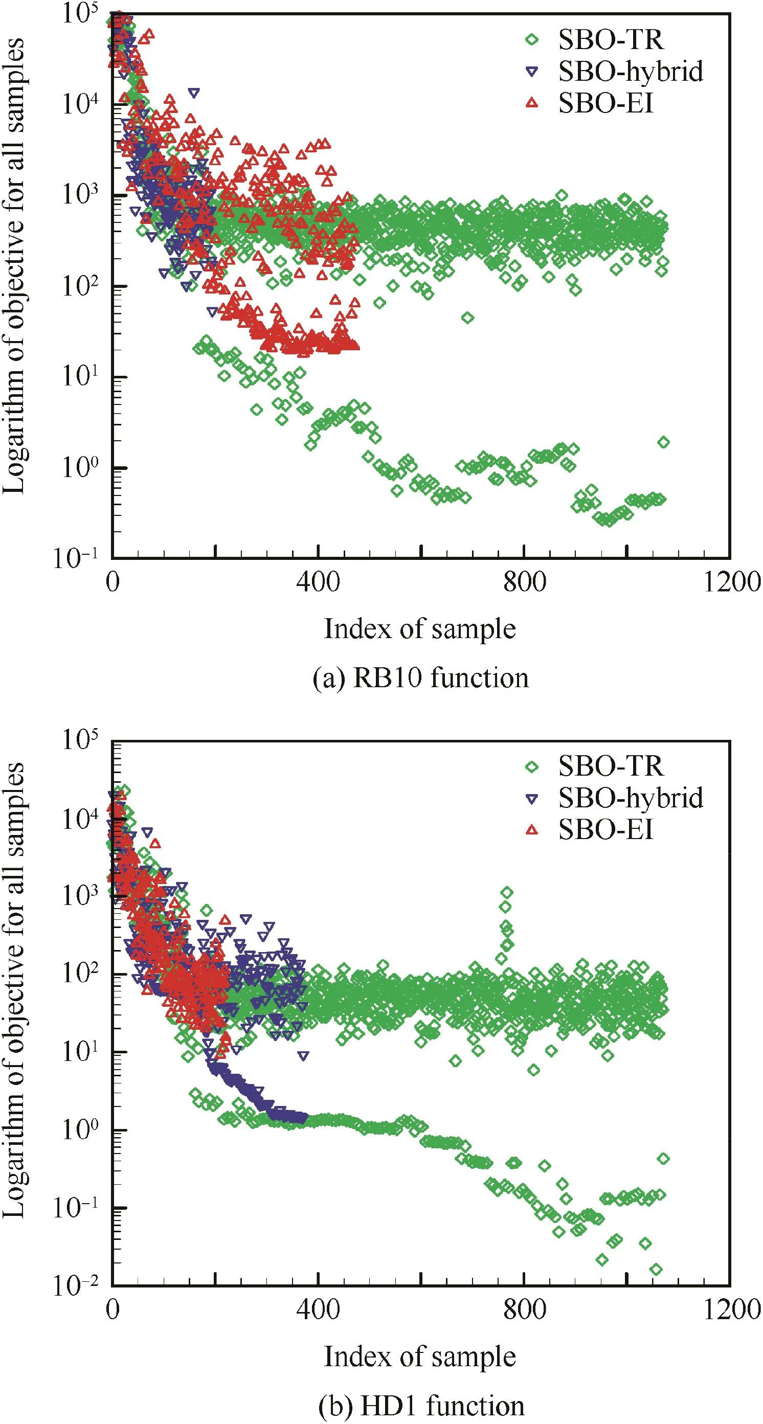
Fig.16 Comparison of objectives for all samples in the databases of the RB10 and HD1 functions.

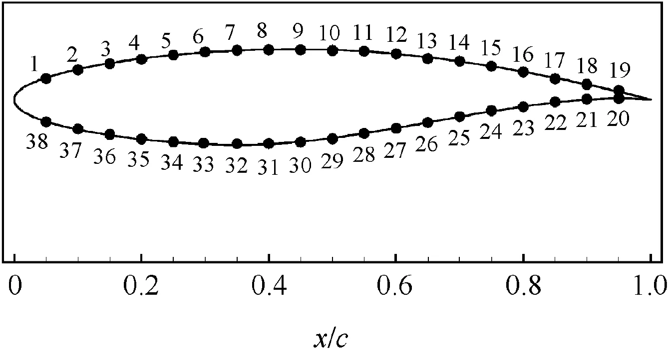
Fig.17 Parameterization of the RAE2822 airfoil.

Fig.18 Hybrid mesh for the RAE2822 airfoil.

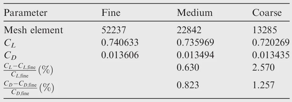
Table 7 Mesh convergence study.

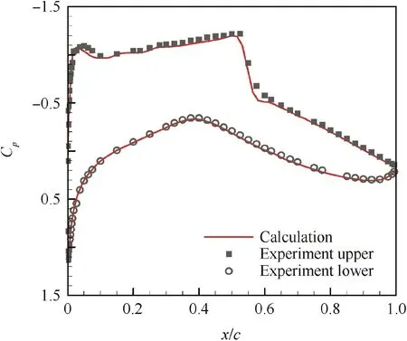
Fig.19 Flow solver validation.

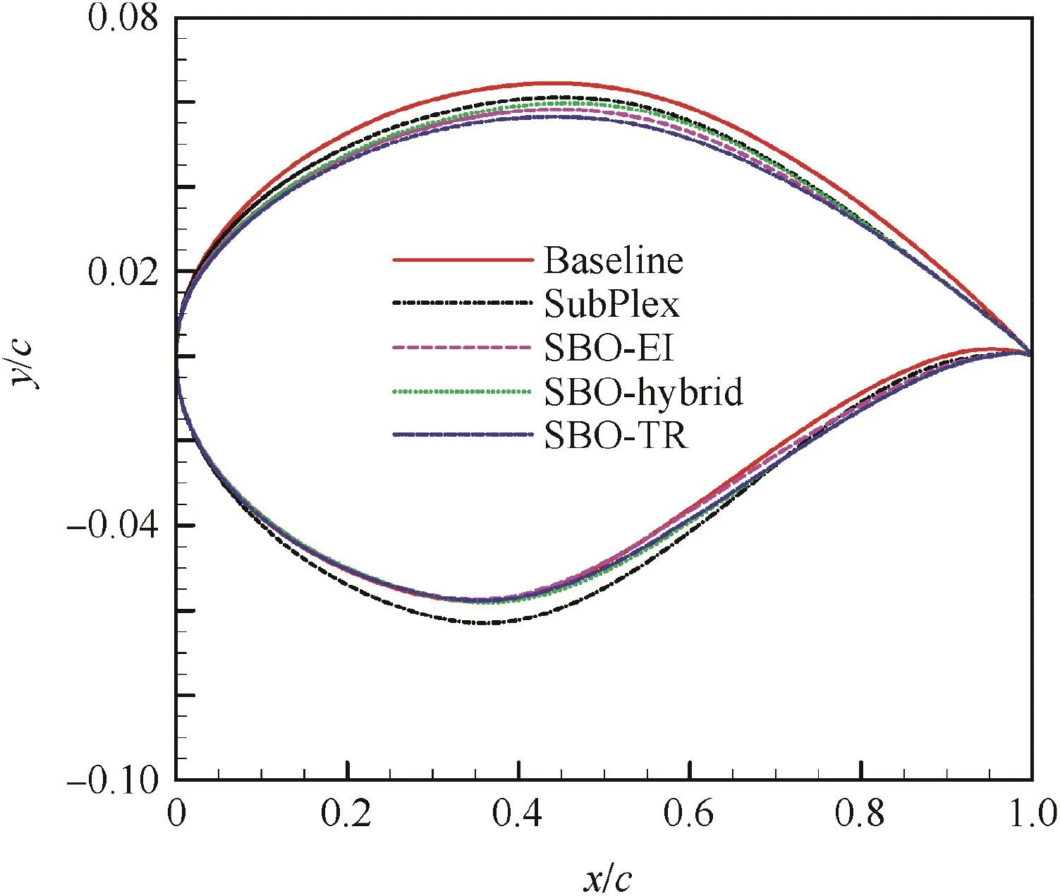
Fig.20 Comparison of geometries.

The optimized geometries and theirCpdistributions are compared respectively in Figs.20 and 21.The strong shock of the baseline geometry has been weakened obviously.Of all the optimized geometries,the one by SBO-TR has the weakest shock,which corresponds to the much flatter upper surface of the geometry(double-dot curves).

The pressure contours around the baseline geometry and the optimized geometry by SBO-TR are compared in Fig.22.A strong shock can be seen on the upper surface of the baseline geometry.In comparison,the shock is smeared on the upper surface of the optimized geometry.It indicates that the drag of the RAE2822 airfoil has been effectively reduced by optimization design.

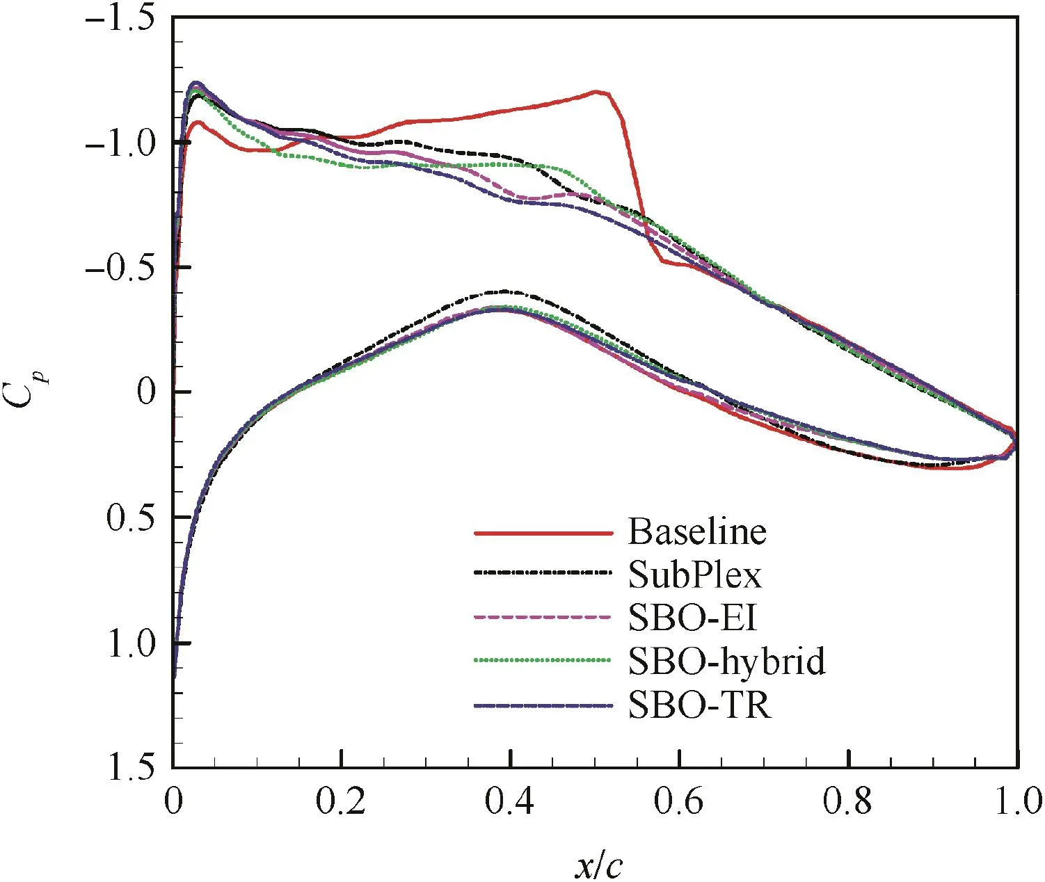
Fig.21 Comparison of pressure coefficients.

Fig.22 Comparison of pressure contours around the baseline and optimized geometries.

Results by using different optimization methods are compared in Table 8.The drag coefficients for all the optimized geometries have decreased.In comparison,the optimized geometry by SubPlex obtains a descent of 28.78 drag counts,while each optimized geometry by the SBOs reaches a little smaller drag coefficient.Among all the SBOs,SBO-TR acquires the largest descent of 33.39 drag counts,but at expense of more CFD analyses.It indicates that SBO-TR can especially enhance the local accuracy of the model.

Table 8 Results of optimizing the RAE2822 airfoil.

4.Conclusions

(1)An optimization methodology with adaptive refinement has been developed by introducing the trust region method into a basic SBO process in this paper.The method is validated and assessed by four analytical tests,and then is applied in drag reduction for an RAE2822 airfoil.

(2)A study of the parameters specified in the SBO-TR process indicates:increasingc2for computing the scale factor of the trust region method is in favor of optimization quality and robustness;c1=0.75 andc2=1.25 are recommended for common problems,whilec1=0.55 andc2=2.00 for strong nonlinear problems;a limit factor of 0.05 for the trust-region radius is recommended.

(3)Results of the tests indicate:in comparison with SBO-EI and SBO-Hybrid,SBO-TR behaves better in local exploitation;although it can most of the time find the global optima for current tests,due to an initially large trust region,SBO-TR is a local-search optimization.

(4)In future work,EI-based refinement could be combined with TR-based refinement,which is supposed to guarantee an efficient global optimization process.

Acknowledgements

This study was co-supported by the National Natural Science Foundation of China(No.11502209)and the Free Research Projects of the Central University Funding of China(No.3102015ZY007).