Scale adaptive simulation of vortex structures past a square cylinder ＊

Javad Aminian

Faculty of Mechanical and Energy Engineering, Shahid Beheshti University, Tehran, Iran

Abstract: The scale adaptive simulation (SAS) turbulence model is evaluated on a turbulent flow past a square cylinder using the open-source CFD package OpenFOAM 2.3.0. Two and three-dimensional simulations are performed to determine global quantities like drag and lift coefficients and Strouhal number in addition to mean and fluctuating velocity profiles in the recirculation and wake regions. SAS model is evaluated against the Shear Stress Transport k-ω (SST) model and also compared with previously reported results based on DES, LES and DNS turbulence approaches. Results show that global quantities along with mean velocity profiles are well-captured by 2-D SAS model. The 3-D SAS model also succeeded in providing comparable results with recently published DES study on Reynolds shear stress and velocity fluctuation components using about 12 times lower computational cost. It is shown that large values of the SAS model constant result in too dissipative behavior, so that proper calibration of the SAS model constant for different turbulent flows is vital.

Key words: Scale adaptive simulation (SAS) turbulence model, bluff body, mean and fluctuating properties, anisotropic turbulence,computational costs

Introduction

Study of flow over bluff bodies is important due to presence in many industries such as buildings and bridges, towers and chimneys, aircrafts, cars and submarines. Aviation and automobile industries always have a passion of drag reduction in order to reducing fuel consumption. In chimneys and buildings, vortex shedding phenomenon plays an important role in the design stage. Fluctuating forces of vortex street which are transverse to the fluid flow may cause resonance leading to the destruction of infrastructures in some cases. Most of these industrial and municipal structures could be studied as simplified square or circular bluff bodies. In recent decades, considerable experimental and numerical studies were conducted to determine characteristics associated with the flow past circular bluff bodies[1]. Fewer works conducted on square cylinders showed that the wake region of flow is wider leading to the Strouhal number being slightly lower than that in circular cylinders[2]. Furthermore,for circular cylinders there is no specified location for separating of the flow, whereas for square cylinders separation points are fixed at the leading edges and upstream corners, this in turn leads to difference in dynamic behavior of the characteristics of the flow field for square cylinders.

Durao et al.[3]performed an experimental study to determine the nature of turbulent flow around a 2-D square cylinder at a Reynolds number of 14 000 using the laser Doppler velocimetry (LDV) technique. They obtained valuable information about Reynolds stresses components in the wake region behind the cylinder and showed that turbulent oscillations allocate about 40 percent of total energy due to high velocity fluctuations.

Saha et al.[4]carried out an experiment to measure two-components of velocity in the wake of a square cylinder using a hot wire anemometer at Reynolds numbers of 8 700 and 17 625. They concluded that profiles of turbulent shear stress are similar to the kinetic energy profiles. They also showed that energy transfers from the mean flow to the streamwise fluctuating velocity in the wake region behind the cylinder.

Using the two-component LDV technique, Lyn et al.[5]have analyzed the characteristics of flow around a square cylinder at a Reynolds number of 21 400. They showed that turbulent length scales and Reynolds stresses are larger than that in circular cylinders and demonstrated that Reynolds stresses are higher in the regions of peak vorticity. They also reported valuable data including time-averaged profiles of mean and instantaneous components of the velocity related to both of the longitudinal and lateral directions as well as global parameters such as the Strouhal number,vortex shedding frequency and drag coefficient. This experimental campaign has received many attentions for validation of several numerical studies because of the number and accuracy of the dataset.

So far, most numerical studies on the Lyn et al.experiment have focused on the Reynolds-averaged Navier-Stokes (RANS) and large eddy simulation(LES) approaches[7-11]. RANS approach is the backbone of CFD simulation with affordable computational cost to model almost all scales of turbulence from micro scales to industrial geometries for which mean quantities are mostly interested. However,RANS techniques are less accurate for flows that contain large separation regions like the wake zone behind bluff bodies. For instance, RANS techniques tend to overestimate recirculation length which is largely affected by high frequency turbulent eddies. It is believed that this behavior is rooted in the nature of the time averaging procedure of the RANS approach.

Direct numerical solution (DNS) is another numerical approach which resolves directly all of the turbulent length scales down to the Kolmogrov length scale. In order to consider details of all fine scales,DNS requires very fine grid, even for low-Reynolds flows in simple geometries. Very recently, Trias et al.[6]have studied turbulent flow around the square cylinder of Lyn et al.[5]using the DNS approach. In general, mean and rms velocity and Reynolds stress profiles as well as drag coefficient and Strouhal number were in a good agreement with experimental data. However, similar to most LES studies, streamwise velocity profile has been overestimated by DNS.They also investigated vortical structures like the von Kármán vortex shedding and the Kelvin-Helmholtz instability which have been produced in the wake region and at the leading edge of bluff body, respectively.

An alternative more affordable approach to solve the instantaneous Navier-Stokes equations is the LES.In this technique, large scales which exceed the filter width are resolved directly, while the high frequency small scales that are more dissipative are modeled by various sub-grid scale (SGS) models. However, LES still requires dramatically finer mesh and much smaller time steps compared with RANS approach. As a consequence, the computational cost of LES approach is much higher than that of RANS, so that its application to sophisticated turbulent flows is limited especially for industrial problems. Sohankar et al.[7]investigated the performance of three different subgrid scale models of Smagorinsky, standard dynamic model and dynamic one-equation model on the flow around the square cylinder of Lyn et al.[5]. They showed that the dynamic one-equation SGS model provides best agreement with experimental data with lowest computational cost. Following to this study,Sohankar[8]conducted another LES study to calculate mean and fluctuating quantities like the drag coefficient, turbulent shear and normal stresses and pressure fluctuation in a wide range of Reynolds number from 1×103to 5×106. He demonstrated that the above mentioned parameters encounter slight variations for all Reynolds numbers, especially at Reynolds numbers above 2×104. In contrast, the large scale instantaneous flow structures like the von Kármán vortices were found almost similar. Shen et al.[12]investigated flow past a modified square stay-cable (MSC) for Re=100, 500, 6 000 and 22 000 by using PIV measurements and 3-D LES. Numerical results for the MSC showed a good agreement with the PIV experimental results and the previous published numerical results.

An alternative turbulence approach developed in last two decades is a hybrid RANS-LES method called the detached eddy simulation (DES). In the DES method, boundary layers which are considered as attached flow regions are modeled by RANS approach,whereas LES is employed for resolving turbulent core in detached regions away from walls. Based on turbulent scales, the DES approach defines explicitly a grid limiter upon which solution procedure switches from RANS to LES mode. Studies conducted on this model have shown that there is a potential source of error due to unwanted activation of grid limiter leading to very high sensitivity of the DES approach to the grid quality[13]. In the scope of hybrid methods,much fewer DES studies have been conducted compared to LES and RANS. DES studies of Roy et al.[14]and Barone and Roy[15]are good examples of hybrid models capability for predicting dynamic flow field around square cylinders. In a two-dimensional numerical study, Roy et al.[14]compared a hybrid DES model with four RANS models including the Spalart-Allmaras, k-ω, shear stress transport (SST)and the Wilcoxʼs improved versions of the k-ω model. They reported that all RANS models overestimate the length of recirculation zone, while DES was able to predict recirculation length and drag coefficient as well as velocity components and Reynolds stresses reasonably well. Barone and Roy[15]have focused on the 3-D simulation of the same square cylinder using DES and investigated the effect of mesh resolution to predict various quantities like Strouhal number of the dominant shedding mode and mean characteristics of the flow in the near-wake region. They showed that prediction accuracy of most parameters can be improved by increasing of grid density. However, for some quantities like the Reynolds shear stress in near-wake region, coarse grid represented better agreement with experimental data.Xu et al.[16]have investigated turbulent flow around a circular cylinder using several turbulence models, i.e.,dynamic sub-grid scale (SGS) model in LES, the Spalart-Allmaras (S-A) and k-ω Shear-Stress-Transport (SST) models in DES, and the S-A and SST models in Unsteady Reynolds-averaged Navier-Stokes(URANS) approach. In general, results obtained by the LES and DES were in good agreement with the experimental data while the URANS showed weak manner to give reasonable results.

Wei et al.[17]have developed a non-linear eddy viscosity model (NLEVM) and a scalable hybrid RANS-LES model to simulate complex flows featuring separations and unsteady characteristics. Flow simulations around a triangular cylinder indicated that the EVM (URANS_SST) was not able to estimate flow characteristics behind the cylinder correctly.However, the non-linear EVM (URANS_SSTNL) was able to improve prediction accuracy to some extent,while the hybrid model based on the NLEVM(Hyb_SSTNL) showed best results in capturing the unsteady behavior due to its scalable feature being adjustable to resolved scales.

The scale-adaptive simulation (SAS) model recently developed by Menter and Egorov[18]is an alternative scale resolving method for capturing dynamic behavior of turbulent eddies with computational cost lower than LES and even DES approaches.Besides the computational cost, the other superiority of the SAS model over the DES approach is that it is not explicitly dependent on the grid size. Therefore,unphysical results at the connecting interface, determined by grid size in the DES approach, are avoided.Derakhshandeh et al.[19]conducted a comparative study on the SST and SAS models to capture complex behavior of unsteady flow around two tandem circular cylinders. They obtained comparable results from both turbulence models in prediction of time averaged pressure coefficient distribution, drag and lift coefficients as well as Strouhal number. However, predictions of SAS were more accurate than that obtained by the SST model. Similar study on tandem spheres has performed by Marchesse et al.[20]to determine the effect of arrangement of several spheres on the pressure distribution and drag coefficient. The accuracy of three turbulence models namely the k-ε,SST and SAS were evaluated against wake extension and pressure coefficient of a single sphere. Results showed inability of the k-ε model in contrast to good agreement of SST and SAS models. Due to closer predictions of SAS results with experimental data on a single sphere, the SAS turbulence model has been used for the study on tandem spheres.

As mentioned above, few studies have focused on complex behavior of fluid flow around square cylinders. Most of them suggested that to improve prediction accuracy for various fluid flow characteristics we have to employ intensive computation approaches like the LES or DES compared to RANS turbulence models. The main goal of this study is to evaluate computational and technical capabilities of the SAS turbulence model on capturing complex behavior of fluid flow around a square cylinder using the open source CFD package OpenFOAM 2.3.0.Toward this goal, besides global quantities such as the drag and lift coefficients, Strouhal number and recirculation length, the mean and rms velocity fields in the wake region as well as Reynolds stresses will be investigated.

1. Configuration and numerical details

In the present study, two and 3-D simulations are performed using the SST and SAS turbulence models to identify flow characteristics past the square cylinder studied by Lyn et al.[5]. They employed a square cylinder of 0.04 m cross section width (D) immersed in a closed water channel. The Reynolds number based on free stream velocity and cylinder width has been kept constant at 21 400. The sketch of problem geometry is shown in Fig. 1. Coordinate origin is chosen at the center of the bluff body similar to the experimental campaign. The computational domain extended 20D in axial direction, including 4.5D before leading edge and 14.5D after trailing edge.Moreover, the computational domain covered 12D in normal direction and 2D in span wise direction.

Fig. 1 Numerical simulation domain in x- y plane

According to Table 1, mesh independency task is performed using three different hexahedral structured grids for both two and three-dimensional simulations.It is worth noting that all results of SAS and SSTsimulations presented in the rest of study have obtained using similar grids as described in Table 1.

Table 1Grid densities in mesh independency task

Time dependent CFD analysis is carried out in a finite volume scheme using the pisoFoam solver available in the open-source CFD package OpenFOAM 2.3.0. As inferred from the solver name, the piso algorithm is used to handle velocity-pressure coupling in flow field equations. Uniform velocity of 1 m/s with turbulence intensity of 2% is specified normal to the inlet boundary. Atmospheric pressure is adopted at the outlet boundary. Zero-shear stress wall is considered at the top and bottom as well as side boundaries. At the bluff sides, standard wall function is employed for turbulence frequency ()ω. Second order discretization scheme is considered for all governing equations. Setting up time-step size equal to 2×10-4s, the Courant number based on the finest cell was obtained about 0.7. Residuals for pressure,velocity, turbulent kinetic energy and turbulent eddy frequency were kept lower than 10-6, 10-6, 10-8and 10-8, respectively. Details of the finest 2-D grid are shown in Fig. 2.

Fig. 2 (Color online) Non-uniform structured grid in the x- y plane

As we know, the SST and therefore SAS turbulence models are relatively insensitive to the local yplus[21]. In particular, for boundary layers with zero pressure gradients it can work equally well with a yplus value of ～1 in the viscous sub-layer or of higher values in the log-law region. However, for flow motions with adverse pressure gradients behind the bluff bodies, applying high quality mesh around the bluff walls could improve solution accuracy. Figure 3 shows the y-plus distribution along the square bluff walls in the fine 3-D SAS case study.

Fig. 3 (Color online) y-plus distributions on the square bluff walls

As can be seen, the y-plus values in both stream wise and transverse directions are less than 32 which correspond to buffer and viscous sub-layers. In transverse direction, the highest y-plus belongs to leading edges on the front wall, while in the stream wise direction the oscillations occurred along the bluff wall.

2. Numerical approach

SAS model is a scale resolving method that can be considered as an evolved version of the Rottaʼs model[22]. Contrary to other two-equation models such as the k-ε and k-ω which deal with heuristic arguments for defining turbulent scale equations (ε or ω), Rotta[22]provided an exact scale-defining equation based on the integral length scale (L) as below

where k represents the turbulent kinetic energy and Riiis the two-point correlation tensor of the velocity fluctuations

The overbar represents a time averaged quantity.Dependence between the three fluctuating velocity components, at two virtual detectors is computed by this tensor. Unity value of R implies a perfect correlation between detectors, while detectors are considered so far apart if degree of correlation tends to zero. For shear flows, Rotta[22]derived a transport equation for the quantity Ψ=kL using Eq. (1). The production term in the transport equation for Ψ contains a mean velocity gradient at the location of second detector according to Eq. (3)

Rotta suggested that the underlying term of integral could be modeled using the Taylor series. Following the assumption of homogeneous turbulence, Rotta assumed that second derivative of the Taylor expansion is negligible (isotropic turbulence for which the two-point correlation R is symmetric) and derived an exact turbulent scale equation based on the first and third terms of the Taylor series[22]

According to Eq. (4), unlike the other twoequation models, the third derivative of the velocity field that can be interpreted as another length scale[23]appears in the model. This term showed the relative ability of the Rottaʼs model, namely the k- kL model, to resolve partly small scales of turbulent spectrum in contrast to classical two-equation models which are reliable mostly in the large scale end.Nevertheless, this term confronts the model with some problems like producing unreasonable results in logarithmic layer of wall[24].

Menter and Egorov have focused on the nonhomogenous flows and recognized that the two-point correlation tensor (R) is asymmetric unlike the homogenous flows[23-24]. They proved that the third derivative of velocity field introduced by Rotta does not have any physical interpretation in the nonhomogenous flows. In return, the second derivative of velocity field must enter the scale-defining equation which resulted in the emergence of von Kármán length scale (LvK) according to Eq. (5):

where κ equals to 0.41. Menter and Egorov introduced their first scale-resolving simulation (SRS)model with a new variable(resembling Ψ in the Rottaʼs model) in the scale-defining equation as KSKL model that is the basis of the SAS model[24-25]:

where the eddy viscosity is defined asand Cμ=0.09, σk=σφ=2/ 3, ξ1=0.8, ξ2=1.47, ξ3=0.0288Length scale ratio (L/ LvK)2appeared in the KSKL model has a key role in detection of flow unsteadiness and determination of turbulent structures with more accuracy. It is demonstrated that this term can be implemented into other classical two-equation models like the SST and give the ability of dynamic behavior to those turbulence models[26-27].

The SST version of k-ω model is a weighted combination of k-ε and k-ω models in a way that the best features of each model emerge[28]. In regions with high Reynolds number, k-ε generally gives acceptable results, whereas k-ω works better in low Reynolds turbulent regions including deceleration and separation caused by adverse pressure gradient. Two transport equations are resolved to obtain turbulent kinetic energy (k) and turbulent eddy frequency ()ω:

where p=τij∂ui/∂xj. One of the main differences between the SST and the standard k-ω models is the cross-diffusion term (last term in Eq. (9)). It eliminates the sensitivity to free-stream values of ω outside of the shear layer that often observed in the k-ω model[28]. However, SST still has the inherent problem of all other RANS models, i.e., high production of turbulent viscosities which in turn causes to predict large length-scales in unsteady regions. The main goal of SAS turbulence model is well resolving of small scales of turbulence via reduced values of turbulent viscosities.

SAS turbulence model includes an additional source term (QSAS) in Eq. (9) compared with SST model[18]

where FSAS=1.25 and ξ2=1.755. The max function and the k-derivative term have been formulated somehow to avoid unphysical results normally obtained by the SST model for boundary layer flows[26].

In the newer version, Egorov and Menter suggested a quadratic form of length scale ratio (L/LvK)2similar to the form in KSKL model (Eq. (7))[29]

Moreover, new values for constants were defined as FSAS=1, ξ2=3.51, CSAS=2. Another feature of the latest version is high wave number damping of turbulent kinetic energy. Analysis of the original version of the SAS model showed that the von Kármán length scale is not only able to adjust itself with resolved scales but also it can reach to dissipative scales namely the Kolmogorov limits. Having no information on the cut-off limit, energy accumulation appears at high wave number which demands very fine grid in the scale of Kolmogorov limits[23]. In the latest version of the SAS model the cut-off limit is defined according to Eq. (12) to limit LvKby the grid spacing Δ[27]

where CS=0. 262 has been calibrated using decaying isotropic turbulence (DIT) and Δ is the cubic root of the control volume size[27]. This limiter is currently employed in the OpenFOAM CFD package for the SAS model. It should be noted that all versions of the OpenFOAM use a combination of Eqs. (10) and(11), shown in Eq. (13), for computation of QSAS.

with similar constants presented in Eq. (10).

Similar to the KSKL model, the term (L/LvK)2is responsible for higher accuracy of the SAS model in unsteady fluctuating eddies compared to the SST model. It is shown that in unsteady regions of flow the von Kármán length scale has smaller value compared to steady regions. For this reason in unsteady regions QSASand following that ω increase which lead to larger magnitude of dissipation term in the turbulent kinetic energy equation (-β*ρωk in Eq. (8)). Eventually based on the definition of νtin Eq. (14) high turbulent viscosity is suppressed[26].

where Ω is the absolute value of the vorticity and F is given by Eq. (15).

Putting in a nutshell, SAS is formulated somehow to act in RANS mode in steady regions and to show LES characteristics in unsteady regions. This behavior occurs automatically in the flow field in a way that if reasonable computational budgets like grid refinement, proper time step size and high order discretization schemes are provide, SAS tends to the features of LES without an explicit switching in the model formulation. Otherwise, SAS reveals the pure RANS characteristics. In other words, SAS turbulence model is applicable to all ranges of Reynolds number in which it acts as a pure low-Reynolds RANS-based model at low computational budgets while provides LES-like computations to capture strong instabilities at high-Reynolds turbulent flows where higher computational budgets are provided. As a result, production of non-physical solutions is avoided by the SAS model. This behavior is different from other hybrid models like the DES which is affected dramatically by the grid resolution. This feature of the SAS model shows high potential for wider use in turbulent flows.In the bluff bodyʼs scope, however, less attention has been paid to the SAS compared to RANS and LES.

3. Results and discussion

3.1 2-D analysis

2-D simulations on three different grids have been performed using the SST and SAS (Eq. (13))turbulence models. Figure 4 shows the mean streamwise velocity for the coarse, medium and fine grids as described in Table 1. As can be seen, in the laminar region before the leading edge all of the velocity profiles overlap while deviations from experiment arise along the wake region after the trailing edge. For both of SAS and SST turbulence models the recovery of velocity profile in the wake region as well as the negative peak velocity has improved with grid resolution.

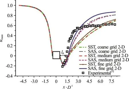
Fig. 4 (Color online) 2-D predictions of mean streamwise velocities (lR is the recirculation length)

As can be seen from Fig. 4, the SST turbulence model shows reasonable results in recirculation zone(0.5＜x/ D＜1.58), while starts to deviate from experiments following to x/ D＞1.5. In particular,the slope of velocity profiles suddenly decreases after recirculation length (lR) in all three grids. However,in all cases, the SAS turbulence model shows enhanced predictions compared to SST model close to recirculation zone (x/ D≤3). Deviation of SAS model from experiment at downstream may come from the three-dimensional nature of von Kármán vortices which requires anisotropic treatment of turbulent structures at x/ D＞3 and will be discussed more in the next section. Instantaneous velocity gradient tensor (Q) is visualized in Fig. 5. According to Eqs. (16) to (18) the Q criterion defines vortices as areas in which the rotation rate (Ωij)magnitude dominates the strain rate (Sij) magnitude(Q＞0)[30].

According to the Q criterion, the vortices developed in recirculation zone (0.5＜x/ D＜1.38) are much smaller than those appeared at downstream. Therefore,fluctuation of small vortices imposes negligible effects on the mean flow field, so that the SST model is capable of capturing mean streamwise velocity in recirculation zone as demonstrated in Fig. 5.

Fig. 5 (Color online) Visualization of turbulent structures by velocity invariant Q=10 colored with mean velocity magnitudes

However, large von Kármán vortices at downstream can greatly affect the mean flow field which is unattainable via RANS approach. As a result,deviation of the SST model from experiment in Fig. 4 has enhanced at downstream. On the other hand,considering vortex fluctuations in turbulent length scale equation (combination of Eqs. (9) and (10))enables SAS model to reasonably capture mean flow characteristics in both recirculation and wake regions(see Fig. 4). Velocity fluctuations in the wake region behind the cylinder are shown in Fig. 6.

SAS model shows closer prediction to experimental data compared to SST for both streamwise and transverse velocities on the same grids. Moreover,grid refinement shows more impact on the SAS predictions compared to SST. Regarding the nonhomogeneous 3-D nature of unsteady vortices, it is expected to obtain more satisfactory results in 3-D anisotropic simulations.

Figures 7 (a), 7(b) illustrate vorticity field obtained using the SAS and SST turbulence models. As can be seen, both turbulence models can predict development of von Kármán Vortex Street behind cylinder. However, a closer look reveals that only the SAS model is able to predict the general repeating pattern of swirling vortices as naturally occurs in classical fluid flow over bluff bodies. It is confirmed by stream-line plots in Figs. 7 (c), 7(d) which demonstrate a frequent pattern attained using SAS turbulence model.

Fig. 6 (Color online) 2-D predictions of fluctuating velocities

Time history of drag and lift coefficients on the finest 2-D grid for SST and SAS turbulence models is shown in Fig. 8.

Results of the SST model show high fluctuations in drag coefficient profile, while cyclic converging fluctuations are obtained using the SAS model. Similar behavior can be observed for the lift coefficient. This behavior may be attributed to unique feature of the SAS model i.e., reducing turbulent viscosity in an effective way. Mean value of drag coefficient reported as 2.1 in the experiment[5]which is reasonably captured by converged uniform result of the SAS model. Due to the flow symmetry and zero attack angle the mean value of lift coefficient must be zero which is accurately predicted by the converged SAS model.

3.2 3-D analysis

3.2.1 Analysis of the SAS model constants

Fig. 7 (Color online) (a), (b) Vorticity fields and (c), (d) stream lines predicted by SST and SAS turbulence models

Fig. 8 (Color online) Comparisons between drag and lift coefficients computed by 2-D SST and SAS

As mentioned earlier, two sets of model constants are suggested for QSASin Eqs. (11), (13).Figures 9, 10 represent the effect of varying coefficients in QSASbased on Eqs. (11), (13) for the mean and fluctuating velocities. From Figs. 9, 10 considerable impact of CSon the mean and fluctuating velocity profiles can be inferred, so that proper calibration of the SAS model constant would be of great interest. Higher values of CScould increase the von Kármán length scale based on Eq. (12) which in turn lead to lower values of the QSASand finally larger turbulent viscosity. This behavior could be seen from Eq. (11) with CS=0.338 in Figs. 9, 10 for which similar pattern to the SST model is produced. It can be seen that the SAS model in the form of Eq. (13)with CS=0.262 shows the best agreement with experimental data compared with other possible cases.Therefore, this case is selected through the rest of study.

Fig. 9 (Color online) Sensitivity analysis on the 3-D SAS model constant (CS) for mean streamwise velocities

3.2.2 SAS model vs. other turbulence approaches

It was shown that 2-D analysis of the SAS model is able to provide reasonable predic- tions not only for global quantities but also for mean streamwise velocity field. Nevertheless, the predicted velocity fluctuations showed great discrepancies with experimental data in 2-D. The mean and fluctuating velocities for the SST and SAS turbulence models together with previously reported numerical results are shown in Figs. 11, 12. By comparing Figs. 4, 6 with Figs. 11, 12, it can be inferred that the SAS model provides enhanced results when switching from 2-D to 3-D simulation. In particular, recirculation length (lR) is poorly predicted by the 3-D SST model, while the SAS model provided reasonable predictions not only for the recirculation length but also for the wake region. Figure 12 shows that the SST model failed to predict both streamwise and transverse velocity fluctuations, while the SAS model provided reasonable results comparable to those of previously reported using LES and DES approaches.In particular, the rms of transverse velocity is well predicted by the SAS approach with minor deviations on the peak position. Similar trend could be observed for the rms streamwise velocity, although the peak value is partly overestimated.

Fig. 10 (Color online) Sensitivity a nalysison the 3-DSAS modelconstant (CS) forstreamwiseandtransvers fluctuating velocities

Fig. 11 (Color online) 3-D predictions of mean streamwise velocities

As mentioned in previous section, the constant CShas an important role in the SAS model. Therefore, dynamic computation of CSbased on the information provided by the resolved scales of motion might enhance rms velocity predictions. Since, for the 2-D and 3-D analysis similar number of grid elements have been employed in the x- y plane (see Table 1),improvements in prediction of mean and fluctuating velocity profiles could be attributed to the using of 18 elements in the spanwise direction, so that the effect of anisotropic 3-D vortical structures on the flow field could be considered in the 3-D SAS simulations.Comparing Figs. 6, 12 elucidates that switching from 2-D to 3-D simulation has not improving impact on the SST predictions which is attributed to the assumption of isotropic turbulence. Figures 13, 14 show components of mean and fluctuating velocities in the axial and cross directions at x/ D=1, respectively.

Fig. 12 (Color online) 3-D predictions of streamwise and transverse fluctuating velocities

Fig. 13 (Color online) Mean streamwise (urms) and transverse(vrms) velocities at x/ D=1

From Figs. 13, 14 it can be inferred that the mean and fluctuating velocity profiles are overestimated by the SST model in both streamwise and transverse directions, while the SAS results are in good agreement with experiments similar to those of reported using the DES approach. It is worth noting that all the operating conditions comprising of type and number of grid elements, boundary conditions, discretization schemes and time step size are quite similar in the present SST and SAS simulations, so that the enhanced results of the SAS model could be related to its anisotropic nature arising from addition of QSASterm to the ω equation in the SST model.

Fig. 14 (Color online) rms streamwise (urms) and transverse(vrms)velocities at x/ D=1

Figure 15 compares time-averaged profiles of Reynolds shear stress obtained by the SST and SAS models together with previously reported DES approach. All models succeeded to predict position of the first peak around y/ D=0.75. The magnitude of the first peak which was developed in the shear layer is partly overestimated by the SAS model similar to the DES approach. However, neither the SAS nor DES was able to predict the secondary peak inside the recirculation zone at y/ D=0.25. Lyn et al.[5]have considered contribution of both periodic and turbulent components in this position and stated that the periodic component has a key role in emergence of the secondary peak. Further studies are required to explore the complex nature of the secondary peak.

Fig. 15 (Color online) Time-averaged profiles of Reynolds shear stress at x/ D=1

Fig. 16 (Color online) Iso-surfaces of the second invariant of velocity (Q=10) colored by mean velocity magnitudes

In Fig. 16 instantaneous iso-surfaces of the second invariant of velocity gradient tensor Q are visualized. It can be seen that the SST model can produce only dominant large structures without capturing the formation of small structures. This can be attributed to its too dissipative property which means that the SST tends to quickly vanish small unsteadiness due to overestimation of turbulent viscosity. On the other hand, results of the SAS model show distinguished enhancements in terms of resolving small structures in the wake region behind the cylinder. As can be seen from the close up figures,3-D SAS model is able to predict appearance of small vortices developed in the shear layer below cylinder caused by Kelvin-Helmholtz instability. In the 3-D SAS calculations, small vortices move down toward the wake region and engulf in the large scale von Kármán Vortex Street.

3.2.3 2-D vs. 3-D SAS results

Results of 3-D SAS model based on Eq. (13)with Cs=0.262 together with two-dimensional SAS model on the fine grid are shown in Figs. 17, 18 for mean and fluctuating velocity components. For the mean velocity profile, while the velocity recovery is better captured by the 3-D SAS model, it can be said that both 2-D and 3-D SAS models provided comparable results in the recirculation zone (x/ D＜3).However, the 3-D SAS model illustrated more accurate predictions for x/ D＞3. Superiority of the 3-D SAS model over the 2-D SAS is clear from the fluctuating velocity components illustrated in Fig. 18.It can be seen that the 2-D SAS model partially captured the streamwise velocity fluctuations while completely failed to capture the transvers velocity fluctuations. Therefore, the anisotropic nature of turbulent eddies around the leading edge and towards wake region at downstream are only attainable via anisotropic treatment using the three dimensional SAS model.

Fig. 17 (Color online) Comparison of the 2-D and 3-D SAS results on mean stream wise velocities

3.3 Computational costs

In the present study, computations are conducted on a cluster of 32 cores (AMD 2.8 GHz), part of a 10 Tflops performance cluster with 640 core and 128 GB RAM. Solution of 6 equations comprising of the continuity, x, y and z velocity components and turbulence parameters k, ω and QSAS(in the SAS model) for 6 s of flow time on a similar grid with 693 k cells took about 1 531 min for SST model and 1 591 min for SAS model. Comparable numerical costs of the SAS model with its original SST model,while providing detailed information on small scale vortices, highlight unique advantages of the SAS model. It should be noted that contrary to most previous numerical studies which have proposed an extended spanwise length, i.e., A=4D, to allow correct formation of 3-D structures, in the present study satisfactory results have also obtained with A=2D.

Fig. 18 (Color online) Comparisons of 2-D and 3-D SAS results on streamwise and transvers fluctuating velocities

3.3 Computational costs

In the present study, computations are conducted on a cluster of 32 cores (AMD 2.8 GHz), part of a 10 Tflops performance cluster with 640 core and 128 GB RAM. Solution of 6 equations comprising of the continuity, x, y and z velocity components and turbulence parameters k, ω and QSAS(in the SAS model) for 6 seconds of flow time on a similar grid with 693 k cells took about 1 531 min for SST model and 1 591 min for SAS model. Comparable numerical costs of the SAS model with its original SST model,while providing detailed information on small scale vortices, highlight unique advantages of the SAS model. It should be noted that contrary to most previous numerical studies which have proposed an extended spanwise length, i.e., A=4D, to allow correct formation of three-dimensional structures, in the present study satisfactory results have also obtained with A=2D.

Spectral analysis (fast Fourier transform (FFT))of lift coefficient is investigated for the finest grid in the SAS model and the frequency of peak sound pressure level (SPL) which is recognized as vortex shedding frequency over the bluff body (f) is employed to determine the Strouhal number (St=). Table 2 compares global quantities such as Strouhal number, drag coefficient and recirculation ratio obtained from present study with experimental data as well as previously reported numerical results.

It can be observed that for global quantities, the low intensive SAS computations, even in two dimensions, can provide comparable results with recently published high intensive LES and DNS computations.The importance of this comparison becomes clearer when we inspect corresponding computational costs presented in Table 3. Recalling from Figs. 11, 12 it can be seen that three dimensional SAS model can provide reasonable results on fluctuating unsteadiness with about 50% lower computational cost comparing with similar LES study conducted by Sohankar et al.[7].Comparing with DES study of Baron et al.[15], it can be seen that the three dimensional SAS model succeeded in providing reasonable results using about 12 times lower computational resources.

Despite the success in describing unsteady small scale local vortices in bluff body scope, the SAS turbulence model requires further tests and refinements to verify its wider applicability for other scopes,conditions and applications.

4. Conclusion

Turbulent flow around a square bluff body was analyzed by two and 3-D simulations using two turbulence models namely the k-ω SST and SAS in the open source CFD package OpenFOAM 2.3.0. In 2-D analysis, the SAS turbulence model showed a better agreement with experimental data in prediction of global quantities like drag and lift coefficients and Strouhal number comparing with the SST model.Nevertheless, both models were incapable of providing reasonable accuracy for fluctuating velocities in 2-D analysis. In 3-D mode, SAS model showed significant enhancements not only in prediction of mean velocity profiles but also in the fluctuating velocities, while the SST model revealed poor resultssimilar to those obtained in 2-D mode. It is shown that the constant CShas an important role in the SAS model. Further studies required to enhance the rms velocity predictions by dynamic computation of CSbased on information provided by the resolved scales of motion. Acceptable performance of the SAS model in the prediction of various mean and fluctuating characteristics along with lower computational cost compared to LES and DNS approaches could place SAS model into attractive turbulence models for CFD studies even in industrial scales which demand affordable computational costs with satisfactory precisions.

Table 2 Comparison of global quantitates

Table 3 Computational grid for 3-D simulations

Acknowledgement

This work was supported by the Research Center of the Shahid Beheshti University (SBU). We are thankful to the SBU cluster “SARMAD” officials which provided access to a high performance computing system.