Finite element analysis of nitric oxide (NO) transport in system of permeable capillary and tissue ＊

Ya-jie Wei (魏雅洁), Ying He (贺缨), Yuan-liang Tang (唐元梁), Li-zhong Mu (母立众)

School of Energy and Power Engineering, Dalian University of Technology, Dalian 116024, China

Abstract: The endothelial dysfunction and the unbalanced secretion of vasoactive substances are the main causes of the macro and micro vascular complications for patients with diabetic mellitus (DM). This paper investigates the blood flow and the nitric oxide(NO) transport in a permeable capillary by using a finite element method. The computational domain consists of a permeable straight or bifurcated capillary and the surrounding tissue with different endothelial hydraulic permeability. The blood flow in the lumen of a capillary is assumed to be governed by the Stokes equation. The fluid flow in the surrounding tissue is simplified as the Darcy flow.The advection–diffusion reaction equation is employed to investigate the NO distribution in a lumen-tissue model, which is originated from the endothelial cells inside the capillary wall. The characteristic Galerkin method is employed for the discretization of the advection-diffusion reaction equation. The simulated results show that the NO transport is effectively affected by different hydraulic permeabilities due to the changes of the blood velocity. When the hydraulic permeability increases considerably, the NO concentration ([NO]) in the whole domain decreases accordingly. Moreover, the NO concentration increases in the area after the bifurcation of the capillary owing to the convective effect. It is also shown that even if the NO production by the endothelial cells is enhanced, the increase of the convection inside the vessel may reduce the endothelial NO concentration. As a signal transduction molecule, the spatial location with discriminating NO distribution may be useful for determining the position of the microangiopathy in the DM.

Key words: Hydraulic permeability, mass transport, finite element method, wall shear stress, Nitric Oxide

Introduction

It is widely accepted that patients with the DM would suffer from the endothelial dysfunction and related alterations of the hemodynamic parameters,including the permeability, the viscosity and the pressure[1-2]. Recently, a number of studies show that the change of the glycocalyx structure under the hyperglycaemia can lead to an increase of the vascular permeability to water[1]. Moreover, the platelets in the diabetic patients show the features of the enhanced adhesion to the endothelium and the effortless aggregation. Due to the change of these parameters,the flow resistance increases to lead to abnormalities of the microcirculation[2]. It is indicated that with the increase of the hematocrit and the stiffness of the erythrocytes, the aggregation of platelets is enhanced[3]. The blood flow in the microcirculation patients with the DM is an issue of great importance as it is related to the early diagnostics of the microcirculation complications of the DM patients.

The NO is functioned as a signal transduction molecule to mediate a variety of physiological processes in the microcirculation. The NO released from the endothelium is identified as a key regulation factor of the vascular tone[4]. In addition, the NO also plays a significant role in the regulation of the platelet adhesion and aggregation[5], the cell-leukocyte interactions and the smooth muscle cell proliferation.Most importantly, the inhabitation of the NO synthesis in the endothelial cells by the L-arginine increases the permeability of the microvessel. Furthermore, the NO originated from the coronary endothelium takes part in the regulation of the myocardial contractile function and in the myocardial energetic activities in the heart.Through inhibiting the proliferation and migration of smooth muscle cells, the NO can protect arteries from developing atherosclerosis[6]. It is revealed that the endothelium-driven NO is related with the neurotransmission as well[7].

In response to neural, vascular and agonist stimuli, the NO is produced endogenously in the body through the enzymatic degradation of the L-arginine by the enzyme NO synthase of several isoforms. It is demonstrated that the endothelial cells are the most important location to produce the NO and the production rate of the NO released from this position depends on the wall shear stress (WSS) on the vascular surfaces. Moreover, there are some other places where the NO can also be produced after the immunological stimulation, including platelets, macrophages and neutrophils. Hence, the production of the NO is closely associated with the blood flow in the vasculature. Once the NO is released from the vascular endothelial cells, it can be diffused into the vascular wall, the tissue and the vascular lumen.When it is diffused across the cell membranes to the adjacent target smooth muscle cells, the NO can activate the soluble enzyme guanylyl cyclase so as to increase the intracellular cGMP (the cyclic guanosine monophosphate concentration) and play its vessel regulatory role[4]. As a small diatomic molecule, the NO can diffuse freely and can be carried away by the fluid. Moreover, the NO can be degraded in various reactions in the process of the transmission. It can react fast with the superoxide and heme-containing proteins such as the hemoglobin, the myoglobin, the guanylate cyclase and the cytochrome C oxidase in vivo[8-9]. Above all, it is well recognized that the process of the NO transport in the vessel lumen, the vascular wall and the tissue is affected by the convection, the diffusion and the reaction.

Numerous mathematical models were adopted to simulate the diffusion of the NO. Vaughn et al.[10]found that both the sizes of the arteriole and the hemoglobin degrading the NO are important factors for the effective distance of the NO diffusion in the microcirculation. With a 3-D microcirculatory network containing two arterioles and nine capillaries,Chen et al.[11]simulated the NO transport in the tissue and found that the red blood cell (RBC) distributions in arterioles and the blood velocity profiles affect the NO distribution significantly. It is a common interest to investigate the factors that influence the NO diffusion in and around arterioles since they are closely associated with the fact that the arteriolar wall is the optimal sites to regulate the blood flow and for the NO to play the vasodilatation role in the arteriolar efficiently. On the other hand, Liu et al.[12]pointed out that the prediction of the NO transport in large arteries,such as the thoracic aorta, may be useful for the detection of the localized region easily inducing and developing the atherosclerosis since one of important physiological functions of the NO is to protect the arteries from producing and developing the atherosclerosis. It is noteworthy that the capillary network forms an NO source for the NO transporting to the arteriolar wall owing to the abundance of the endothelial cells in the capillary wall. Through the observation of the capillary response to the local application of the NO synthase inhibitor and stimulator using the intravital microscopy, Mitchell and Tyml[13]revealed that the low basal levels of the NO affect the capillary blood flow by modulating the local hemoconcentration and the leukocyte adhesion and the high levels of the NO may cause a remote vasodilation to increase the microvascular blood flow.In view of the above facts, Nikolaos and Popel[14]estimated the NO exchange and concentration level in the system of the capillary and the tissue, and the results can be used to investigate the NO diffusion around arterioles.

Although the characteristics of the NO transport were much studied, the influence of the convection during the transport is often ignored and a constant NO production rate (RNO) is assumed in the studies[14-15]. It is demonstrated that the NO produced by the endothelial cells is influenced by the WSS at the surface of the vascular wall, which is related to the blood flow in a vessel. On the other hand, the change of the fluid velocity in the vascular lumen or through the interstitium in the tissue affects the NO transport process significantly[12,15-16]. Recently, Liu et al.[15]computed the flow field in the arterial lumen with a stenosis and the arterial wall based on the Navier-Stokes equations and the Darcyʼs Law and obtained the NO distribution with considerations of the advection–diffusion reaction equation. Their model focused on the NO transport influenced by the flow disturbance in a large artery. Fadel et al.[16]and Plata et al.[17]theoretically investigated the endothelial NO production and transport in parallel plate flow chambers. They found that the enhanced NO production by the endothelial cells and the increase of the blood flow have a negative effect on the endothelial NO concentrations. However, in their computational models, a simple flow field such as that with a parabolic or plug velocity profile was assumed, which may not reflect the complex flow conditions in the NO transport, such as the flow in permeable vessels.

With many pores distributing in the endothelium,the capillary walls work as semi-permeable walls,where the water can diffuse freely, while the transmission paths of the ions and the macromolecules are impeded selectively. Thus, the characteristics of the NO transport in and around the capillary are very much affected by the seepage flow. This paper explores the change of the NO concentration induced by the flow field with different permeable coefficients of the vascular wall. Because the NO can regulate the permeability of the microvessel to the water and the proteins and the platelet adhesion and aggregation, a model, consisting of the permeable capillary with different hydraulic permeabilities and the tissue, is applied to compute the NO transport.

1. Method

1.1 Governing equations

1.1.1 Fluid dynamics

Lumen: In the microcirculation, the Womersley number of about 0.01 is so small that the pulsating effect can be ignored and the flow can be considered as a steady flow. Moreover, as the Reynolds number of the microcirculatory system is about 0.002-0.7, the convection term of the blood flow also can be neglected. Thus, the flow simulation with the 2-D mathematical model of the capillary is based on the stokes flow.

The mass conservation in the capillary lumen can be expressed as

where uband pbrepresent the fluid velocity vector and the pressure in the capillary, and μ is the blood flow viscosity (μ=4.0× 10-3Pa· s)[18].

Tissue: The fluid flowing through the interstitium in the tissue, which is assumed to be an isotropic porous medium, can be described by the Darcy equation

The mass conservation in the interstitium can be expressed as

where utand ptrepresent the fluid velocity vector and the pressure through the interstitium in the tissue.κ refers to the hydraulic conductivity of the interstitium, which is calculated as /λ μ. λ and μ represent the permeability and the viscosity of the interstitium, respectively. Because the hydraulic conductivity of the tissue is difficult to be obtained, the permeability of the leather (9.5×10-10-1.2×10-9m2)[19]is used to represent that of the interstitium as a reference. Thus, the range of the hydraulic conductivity for the interstitium is about 2.7×10-11-3.0×10-11m2/Pa·s.In this computation, the hydraulic conductivity is assumed to take the value of κ=10-11m2/Pa· s.

Endothelium: To establish the relationship between the fluid flowing in the capillary and the tissue, the transmural velocity (Je) across the capillary wall (the endothelium) is assumed to follow the Starlingʼs law.

In the above equation, Lpis the hydraulic permeability of the endothelium, pbrepresents the interfacial blood pressure and pinterrefers to the interstitial fluid pressure, respectively. The flow through the pores of the capillary wall is assumed to be the Poiseuille flow. As the inverse of the resistance,the hydraulic permeability can be expressed as

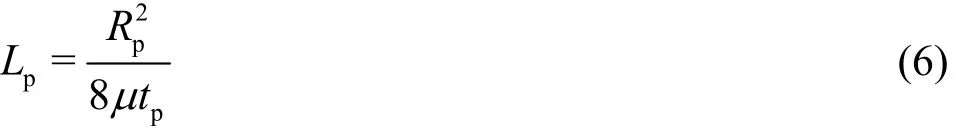
where Rpand tpare the radius and the thickness of the pores in the capillary wall, respectively. The radius and the thickness of the pores are normally assumed to be 4×10-3μm and 0.5 μm. From the above equation, the hydraulic permeability Lpof a normal vessel wall is about 10-9m2/Pa·s, thus the hydraulic permeability is assumed to take a value in the range of 10-10-2.0×10-7m2/Pa·s in our study.

1.1.2 NO dynamics

Lumen: The NO transport in the capillary is mainly determined by the following transient diffusion-convection-reaction equation.

where cbis the NO concentration in the capillary,Dbis the diffusion coefficient of the NO in the blood and takes a value of 3.3×10-9m2s-1[1], and ubis the fluid velocity vector in the capillary.represents the NO reaction rate with the oxygen and the hemoglobin in the RBCs in the capillary lumen, which can be described by the following equation

Since the NO is chemically reacted with the oxygen and the water, the kinetics of the NO auto-oxidation are assumed to be of the third order.Thus, the NO reaction rate with O2is written as

where co2is the oxygen concentration in the aqueous medium and k3is the third order NO auto-oxidative reaction rate. Since c (c～10-3M) is signifi

o2o2cantly larger than cb(cb～10-6M), it is assumed that the oxygen concentration in the fluid remains constant in this study. Therefore, the NO autooxidation can be represented by a psuedo-secondorder reaction.

where koxygenis the psuedo-second-order reaction rate (7.56×10-6nM-1s-1)[17].

The second term on the right hand side of Eq. (8)represents the NO concentration scavenged by the hemoglobin in the RBCs, and it is well demonstrated that the hemoglobin is an effective scavenger to the NO in the blood[11]. The clearance rate by the RBCs can be described by the following equation

where k2and krbcrepresent the second- and firstorder reaction rate constants. cHbis the hemoglobin concentration in the capillary and that in the blood is assumed to be 2.3 mM in this study. The effective second-order rate constant between the NO and the hemoglobin encapsulated RBCs is about 103-105M-1s-1[20], thus the variation range of krbccan be computed as 2.3-230 s-1. The value of krbcis set to 23 s-1in this simulation.

Tissue: The transport of the NO in the tissue is mainly determined by the following transient diffusion-convection equation:

where Dtis the diffusion coefficient of the NO in the tissue and takes a value of 3.3×10-9m2s-1. ctrepresents the local concentration of the NO in the tissue, and utis the fluid velocity vector in the interstitium of the tissue. ktrepresents a pseudofirst-order reaction rate constant of the NO in the tissue, which is set to 1 s-1.

Endothelium: We use a hyperbolic model to calculate the WSS-dependent RNOin this study[21]. In the hyperbolic model, RNOcontains two terms: a constant basal production and a WSS-dependent term.The specific equations to calculate the WSS and NO productions are as follows:

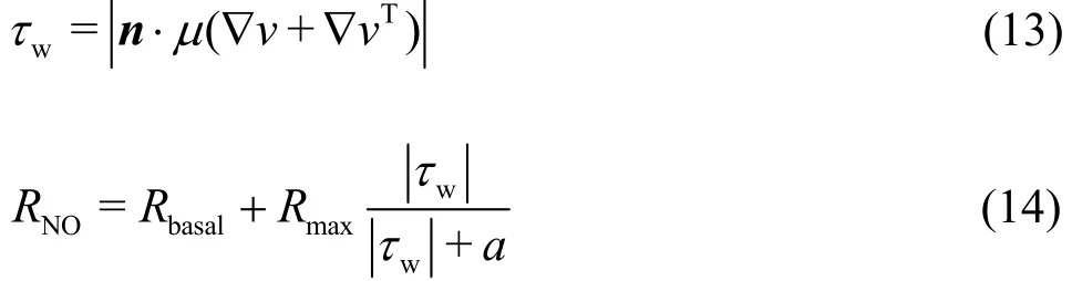
In Eq. (13), n represents the normal vector to the endothelial surface and T is the transpose operation.Rbasaland Rmaxare the basal and maximum RNO,which are set to 2.13 nM/s and 457.5 nM/s,respectively. The parameter a is the wall shear stress corresponding to the half of the maximum RNO,which is set as 3.5 Pa.

1.2 Numerical method

The governing equations are discreted by the finite element method (FEM). The FEM is well suitable for analyzing the heat transfer and the fluid flow in complex geometries. With the arbitrary variation of the shape and the density of the element,the simulated results could meet the demands with a small number of nodes.

The transfinite interpolation (TFI) method is employed for the mesh generation. The domain is first divided into several sub-domains, and the meshes in each sub-domain are generated via the TFI method subsequently. Finally, a whole computational domain with precise grids is assembled from the sub-domains.In the computation, the domain containing a straight vessel and the surrounding tissue is divided into three sub-domains and the mesh spacing along the axial direction of the vessel is 8.75 μm. The mesh spacing along the radial direction of the capillary and the tissue is 1.0 μm.

The computational domain with a bifurcated vessel is divided into five subdomains and the mesh generation is carried out in every one where the mesh spacing takes values in an arithmetic series along the flow direction of the main vessel. The employed mesh spacing inside the vessel is 1.0 μm. The adaptive mesh spacing can be easily controlled by using this method.

Equations (1)-(4) are discretized by using the Galerkin method and the computing procedures are shown in our previous paper[22]. If the same Galerkin approximation is used in the solution of the NO diffusion-convection-reaction equation, the results might be divergent with spurious oscillations since the element Peclet number exceeds the critical value. In order to reduce the influence of spurious oscillations,many methods were proposed. In this study, the characteristic Galerkin (CG) approach is adopted to diminish the spurious oscillations caused by the discretization of the convection terms. Eq. (7) can be transformed as follows

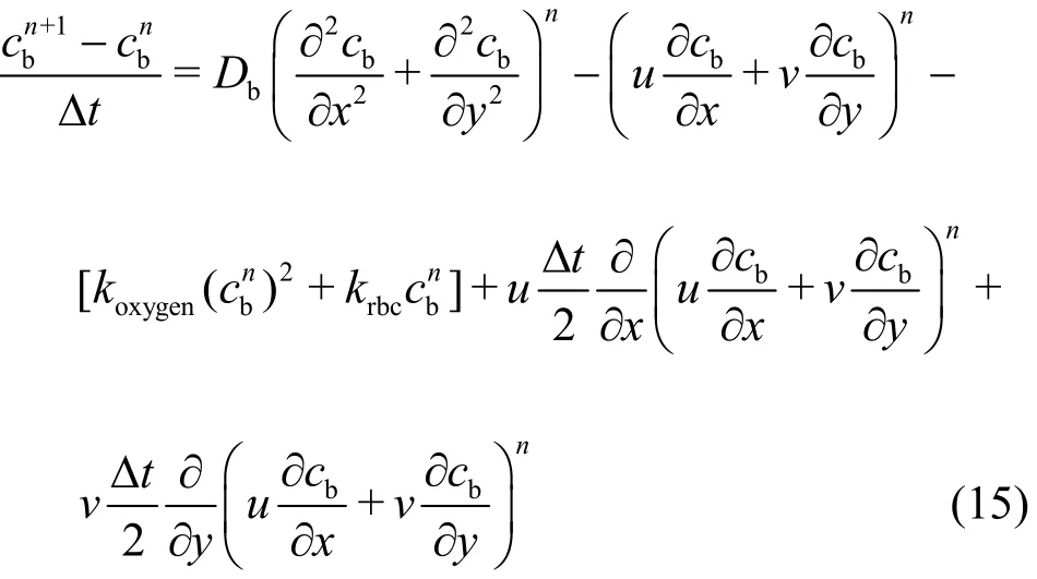
where the 4thand 5thterms in the right-hand side of Eq.(15) are the stabilization terms.

Assuming a liner variation within a triangular element, cbcan be expressed as

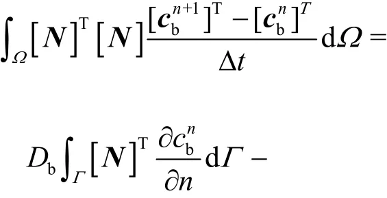
Then, employing Galerkin weighting to solve Eq.(15), we obtain

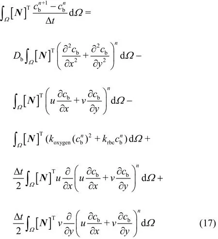
In particular, the Greenʼs lemma is employed to transfer the second-order derivatives in Eq. (17) into the first-order derivatives, thus the diffusion (the 1stterm at the RHS) and the stabilization (the 4thand 5thterms at the RHS) terms can be rewritten as:

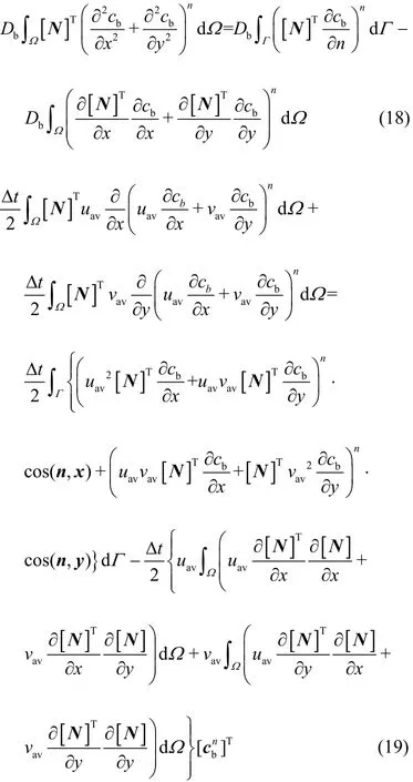
where uavand vavare the average velocities of u and v over an element, which can be computed from the node velocities. In the computation, it is assumed that the boundary integral term in Eq. (19) due to the CG stabilizing operator can be neglected without any loss in accuracy.

Substituting the shape function of cb(Eq. (16)),and Eqs. (18) and (19) into Eq. (17), the finite element equation becomes

The final matrix equation takes the following form after the finite element equations of every element are assembled

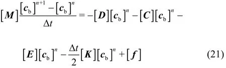
where

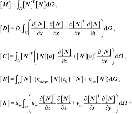
In these expressions, [M] is the consistent mass matrix, [D] is the diffusion matrix, [C] is the convection matrix, [E] is the consumption matrix,[K] is the stabilization matrix, [f] is the forcing term resulting from the second-order diffusion term.

In the same manner, Eq. (12) for the NO transport in the tissue can be discretized. In the computation, the pressure of the domain is obtained simultaneously by using the conjugate gradient (CG)method. Then the velocity is calculated directly using Eq. (1) and Eq. (3). Finally, the NO concentration is calculated explicitly using Eq. (21). The distribution at the time step when the maximal relative residual of the NO concentration for all nodes is less than 10-9is considered to be the one in the steady state.

1.3 Geometry of the computational model

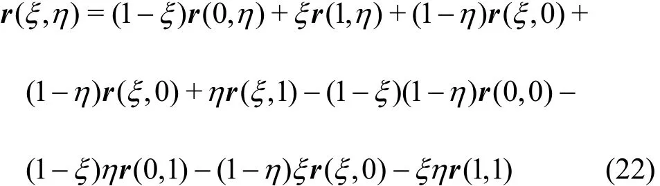
Two geometric models are used to simulate the fluid dynamics and the NO distribution in our study.Figure 1 shows the computational domain with a straight vessel and the surrounding tissue. We ignore the effect of the thickness of the endothelial cells in this simulation. The generated mesh layout of the system of the bifurcated capillary and the tissue is shown in Fig. 2. The formula for the transfinite interpolation (TFI) is expressed as

The geometric parameters of the two models are summarized in Table 1.

2. Boundary conditions

2.1 The boundary condition of fluid dynamics equation

As shown in Fig. 1, since the mean range of the pressure in the capillary network is about 15-40 mmHg[18],the pressures at the inlet and the outlet of the vessel are set to 2 700 Pa and 2 500 Pa, respectively. The pressure at the tissue boundary is set to be equal to that at the outlet of the capillary, which is the same as that assumed by Pozrikidis[23]. At the inlet and the outlet of the interstitial flow, the pressure gradient is assumed to be zero. At the capillary wall, the pressure condition can be written as

The blood and interstitial pressures at the capillary wall can be obtained by calculations in the vessel and tissue domains iteratively. When the pressure in the vessel domain is computed, the interstitial pressure at the capillary wall is assumed to be known.Similarly, when the interstitial pressure in the tissue domain is computed, the computed blood pressure at the capillary wall is given. The iterations are continued until the pressure distribution in the whole domain reaches the steady state.

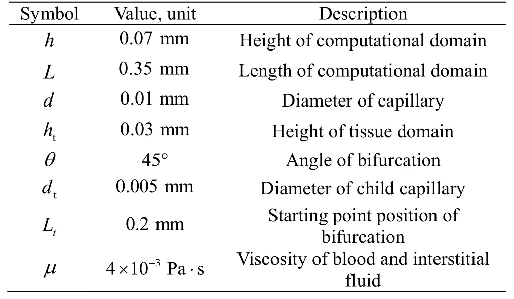
Table 1 Description of the constant parameters used in the simulation

Fig. 1 Schematic diagram of computational domain and boundary conditions

Fig. 2 Generated mesh for a bifurcated vessel by the method of transfinite interpolation

2.2 The boundary condition of NO transport

The NO concentration at the inlet of the capillary is assumed to be 0 nM and the flux of the NO at the outlet of the capillary is assumed to be zero as.

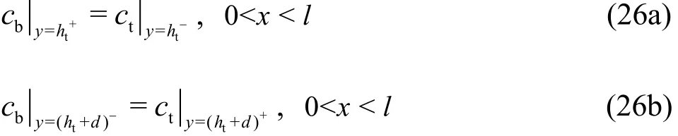
where htis the tissue thickness and d is the diameter of the capillary. The NO concentration across the interface between the capillary and the tissue is assumed to be continuous, which can be expressed as:

The mass flux across the endothelium is assumed to be equal to RNO, which is written as

The first and second terms in the left hand side of Eq.(27) are the NO mass fluxes from the endothelium into the lumen and the tissue. T is the thickness of the endothelium, which is assumed to be 2 μm. RNOis the NO production rate in the endothelium. The NO produced at the capillary wall transports into the capillary lumen and the tissue in diffusion and convection. Thus, the convection term in the element equation (Eq. (20)) should be disposed using the Greenʼs lemma owing to the influence of the endothelial boundary

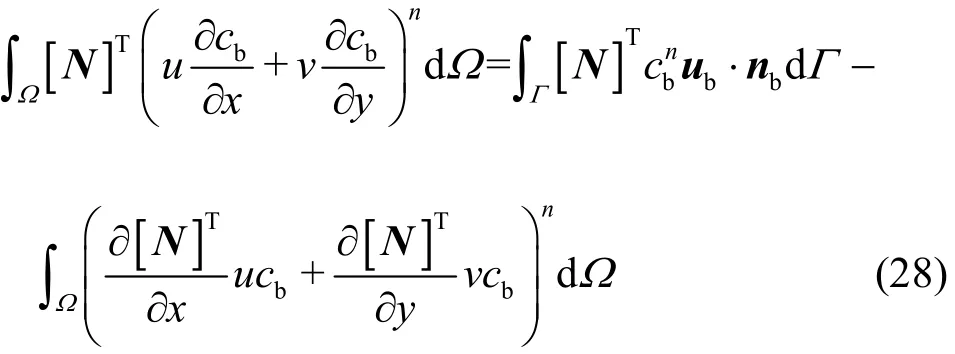
Then, the convection and force matrices [C]and [f]in Eq. (21) with consideration of the endothelial influence become:

In view of the boundary conditions in the other tissue boundaries, the fluxes of the NO in the boundaries are assumed to be zero.

3. Results

3.1 Validation

Prior to the computation of the fluid flow in a permeable capillary and the surrounding tissue, a benchmark test for our computational algorithm is conducted. The fluid dynamics in a combined system of the low permeability porous flow regime and a free flow regime in a confined channel is simulated, whose computational domain (Fig. 3) is the same as that adopted by Hanspal et al.[24]in 2006. Unlike their work, the fluid is considered as the Newtonian fluid in our model. The fluid viscosity is set to 80 Pa·s and the inlet pressure is set to 2.0×105Pa. Other boundary conditions are the same as those in the reference, as shown in Fig. 3. The permeability of the porous media is set to 10-11m2. It is worth noting that there is a membrane connecting the free and porous regions in our model for simulation of the permeable vessel originally. The membrane is set to be almost free so as to let the test close to the case of Hanspal et al..

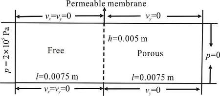
Fig. 3 Schematic diagram of the rectangular coupled free/

Fig. 4 (Color online) Predicted pressure and velocity distributions for the rectangular coupled domain

Figure 4 shows the predicted pressure and velocity distributions in the coupled channel domain. The pressure drop in the Stokes flow domain accounts for 24.1% of the total one, which is close to the percentage computed by Hanspal et al.[24]In the porous media region, the simulated velocity in the flow direction is 2.07897×10-4m/s, which is consistent with the manually computed value of 2.02584×10-4m/s by using the Darcy equation.Meanwhile, the simulated mean velocity in the Stokes flow region is 0.17204 m/s, slightly lower than the value computed by the Poiseuille equation. Thus, the comparison shows the reliability of the code in simulating the coupled Darcy/stokes flow.

Fig. 5 (Color online) Predicted pressure and velocity distributions and NO distributions in the blood and interstitial flow regimes. (a) Pressure and velocity distributions when hydraulic permeability is set to 1.0×10-10 m/Pa·s.(b) NO distribution when hydraulic permeability is set to 1.0×10-10 m/Pa·s. (c) Pressure and velocity distributions when hydraulic permeability is set to 1.0×10-7 m/Pa·s. (d)NO distribution when hydraulic permeability is set to 1.0×10-7 m/Pa·s

3.2 NO transport in the system of straight vessel and tissue

The NO production rate in the endothelial surface is determined by the wall shear stress and the NO distributions inside and outside of the capillary are influenced by convection and diffusion. It was demonstrated that the permeability of the wall affects the flow field considerably in the capillary[25]. To reveal the effect of different hydraulic permeabilities on the NO concentration and the effect of the flow field, we compute the flow field and the NO distribution in the entire domain when the hydraulic permeability is changed from Lp=1.0× 10-10m/Pa· s to Lp= 1.0× 10-7m/Pa· s .

Figure 5(a) shows the distributions of the pressure and the velocity in the blood and interstitial flows. It is seen that the pressure decreases gradually along the axial direction of the whole domain and from the vessel to the tissue boundary along the radial direction. As the interfacial blood pressure is higher than the interstitial pressure in the tissue, the blood can flow out from the capillary to the tissue in the whole domain. In addition, the magnitude of the velocity vectors is reduced slightly along the axial direction due to the seepage of the blood. The distributions of the pressure and the velocity in the whole domain are shown in Fig. 5(c) when the hydraulic permeability is increased to 1.0×10-7m/Pa·s.It can be seen that the pressure gradient increases in the entrance of the capillary, due to the excessive permeation.

Figure 5(b) shows the corresponding NO distribution in the entire domain. The NO is known to be produced by the endothelial cells and it then diffuses to the vascular lumen and the tissue. In the process of the NO diffusion, the blood flow and the consumption by the oxygen and the hemoglobin also influence the NO distribution. We can see from this figure that the concentration of the NO assumes the maximum at the capillary wall and reduces gradually from the endothelium to the tissue boundary along the radial direction. It is noteworthy that the NO concentration inside the vessel lumen is less than that in the tissue due to the excessive consumption. In addition, due to the convection, the NO concentration increases along the axial direction gradually. Figure 5(d) shows the NO distribution when the hydraulic permeability is set to 1.0×10-7m/Pa·s. In this case, the NO level is lower than that when L=1.0× 10-10m/Pa· s . The concen

ptration in the middle region is the highest owing to the effect of the convective transport in the capillary lumen.

3.3 Effect of endothelial hydraulic permeability for no transporting in straight vessel

It is demonstrated that the hyperglycaemia can alter the structure of the glycocalyx covered endothelial surface. Due to this change, the permeability ofthe capillary wall to the water increases remarkably,while the permeability to the protein does not change significantly[1]. The apparent increase of the hydraulic permeability has a profound effect on the distributions of the pressure and the velocity in the whole domain,and further affects the NO distribution.

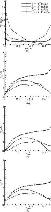
Fig. 6 Effect of different hydraulic permeabilities on (a) WSS variation along the lower wall of capillary. (b) The variation of NO concentration along the lower vascular wall in the axial direction (y=0.03). (c)The variation of NO concentration along the vascular centerline in the axial direc-

There is a positive correlation between the WSS and NO production rates, thus the WSS variation along the vascular wall reflects the NO production rate directly. The WSS and NO distributions along the capillary wall in the axial direction for various hydraulic permeabilities are shown in Fig. 6, while the NO concentration profiles along the radial direction for different hydraulic permeabilities are shown in Fig.7.

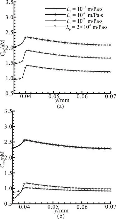
Fig. 7 Effect of different hydraulic permeabilities on (a) the variation of NO concentration in the radial direction near

It is seen from Fig. 6(a) that when the hydraulic permeability ranges from 10-10m/Pa·s to10-8m/Pa·s,the two profiles of the WSS are overlapped and there are almost no differences under the two conditions.The maximum WSS appears at the entrance and the exit of the vessel, which is about 4.5 Pa, while the value of the WSS maintains a value of about 2.3 Pa in the other regions. The distributions of the NO concentration along the vascular wall for various hydraulic permeabilities are shown in Fig. 6(b). Similarly, it can be observed that the NO distributions against the hydraulic permeability ranging from 10-10m/Pa·s to 10-8m/Pa·s see little change. In this range, the highest WSS at the exit of the vessel corresponds to a dramatic growth of the NO concentration value there.However, when the hydraulic permeability increases to 10-7m/Pa·s, the value of the WSS falls monotonically along the vascular wall. In this case, the maximum NO concentration value along the vascular wall is at the location of x=0.1575 mm with a value of about 1.877 nM. When the hydraulic permeability is further increased to 2×10-7m/Pa·s, the excessive pressure drop of the fluid along the vessel results in a reversal flow near the outlet which is not good for the NO transport. Thus, the WSS distribution tends in a shape of parabola with opening upward and the value of the WSS is higher than those in other situations. In this case, the NO concentration variation along the vascular wall takes a similar M shape. Figures 6(c),6(d) show the NO distributions along the vascular centerline (y=0.035 mm)and the tissue (y=0.055 mm). It can be seen that when the hydraulic permeability is larger than the value of Lp=1.0×10-7m/Pa· s , the NO concentration at the capillary wall, the centerline and the tissue are considerably lower than those when=1.0× 10-10m/Pa· s . The concentrations at the capillary wall and the tissue near the exit when=2.0× 10-7m/Pa· s are slightly larger than those when the hydraulic permeability is set to 10-7m/Pa·s due to the appearance of the reversal flow.

Figure 7 shows the NO concentration profiles within the domain with various hydraulic permeabilities along the radial direction. It can be observed from Fig. 7(a) that in the middle of the capillary, the NO concentration inside the capillary lumen is considerably lower than that in the tissue. However, at the position near the exit (Fig. 7(b)), it seems there is no significant difference for the NO concentration inside the lumen and the tissue, due to the convective transport in the whole domain.

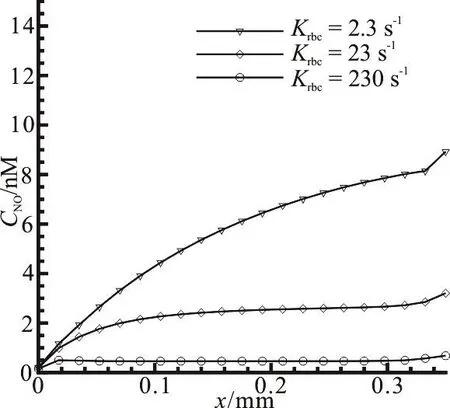
Fig. 8 Effect of reaction rates by red blood cells on NO distribution along the vascular wall

3.4 Effect of hemoglobin in red blood cells for No transporting in straight vessel

The NO can react with the abundant hemoglobin in the RBCs of the capillary fast. The concentration level of the NO in and around the capillary is determined by the reaction rate between the NO and the hemoglobin in the process of the NO transport primarily. Figure 8 illustrates the NO distribution at different reaction rates with the RBCs. It is shown that the NO concentration apparently decreases along the vascular wall when the reaction rate with the RBCs krbcincreases from 2.3s-1to 230, which indicates that the hemoglobin in the RBCs is an effective substance to eliminate the NO in the whole model.

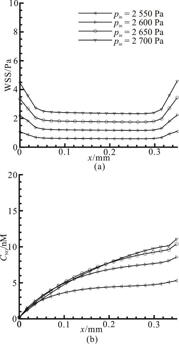
Fig. 9 Effect of the pressures at the inlet of capillary on (a) wall shear stress variation along the capillary wall. (b) NO distribution along the vascular wall

3.5 Effect of the pressure at inlet of capillary for NO transporting in straight vessel

Not only the NO production but also the convection has an impact on the NO distribution. Meanwhile,the NO production and the convective term change with the flow field and the pressure drop. Thus, we compute the WSS and NO distributions along the capillary wall and they are seen to be influenced by the inlet pressure pinwhen krbcand Lpare zero and 10-10m/Pa·s, respectively. As shown in Fig. 9(a),when pinincreases from 2 550 Pa to 2 700 Pa, the WSS monotonously increases and the largest WSS is close to 5 Pa. Fig. 9(b) shows the variation of the NO distribution against different inlet pressures. It is observed from Fig. 9(b) that although the NO concentration increases with the inlet pressure, the increase is not in a linear manner as that of the WSS in Fig.9(a). When pinis increased from 2 650 Pa to 2 700 Pa,the NO concentration at the exit of the capillary is merely increased by 0.69 nM. In addition, the concentration near the inlet is even slightly decreased as compared to the values when the inlet pressures are 2 600 Pa and 2 650 Pa, respectively. According to Eq.(14), the NO production rate increases fast when the WSS is less than 5 Pa. This implies that the convection effect in the vessel lumen becomes stronger to counteract the increase of the NO production when the inlet pressure is larger than 2 650 Pa.

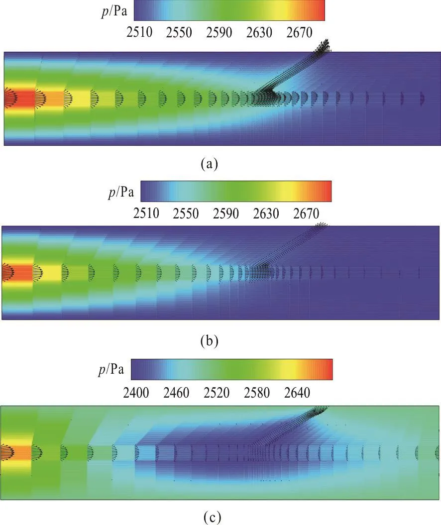
Fig. 10 (Color online) Predicted pressure and velocity distributions at the bifurcated capillary and the surrounding tissue. (a) Pressure and velocity distributions when hydraulic permeability is set to 1.0×10-10 m/Pa·s. (b)Pressure and velocity distributions when hydraulic permeability is set to 1.0×10-7 m/Pa·s. (c) Pressure and velocity distributions when hydraulic permeability is set to 2.0×10-7 m/Pa·s. The pressures at the inlet of the main capillary and the outlets of the two capillaries are set to 2 700 Pa, 2 500 Pa and 2 500 Pa

3.6 NO transport in a bifurcated vessel

In order to investigate the hemodynamics and NO distributions in different vascular structures, we further analyze the NO transport in the system of the bifurcated blood vessel and the tissue. The child vessel starts at the position 0.2 mm away from the entrance of the vessel in the axial direction and the diameter of the child capillary is 5 μm. The bifurcated angle between the two vessels is 30°. The distributions of the pressure and the velocity in the bifurcated blood vessel and the interstitial flow are shown in Fig. 10 for different hydraulic permeabilities (Lp=1.0×10-10m/Pa· s ,L=1.0× 10-7m/Pa· s and L=

pp2.0× 10-7m/Pa· s ), while the NO distributions in the entire domain are shown in Fig. 11 when Lp=1.0× 10-10m/Pa· s and L=1.0× 10-7m/Pa· s .

p

Figure 10(a) shows the distributions of the pressure and the velocity in the bifurcated vessels and the surrounding interstitial tissue when the hydraulic permeability is set to 1.0×10-10m/Pa·s. It is seen that due to the existence of the child vessel, the pressure drop is not as uniform as that in the straight vessel(Fig.5(a)). The pressure drop before the bifurcation is larger than that after the bifurcation. Meanwhile, the velocity in the main branch of the capillary decreases significantly. In addition, Figs. 10(b), 10(c) show the pressure and velocity distributions in and around the bifurcated capillary when the hydraulic permeability is set to 1.0×10-7m/Pa·s and 2.0×10-7m/Pa·s,respectively. It is noteworthy that there appears a reversal flow in the main child vessel when the hydraulic permeability is set to 2.0×10-7m/Pa·s.

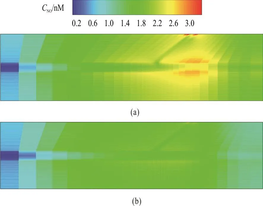
Fig. 11 (Color online) Predicted NO distribution in the system of bifurcated capillary and surrounding tissue. (a) NO distribution when hydraulic permeability is set to 1.0×10-10 m/Pa·s. (b) NO distribution when hydraulic permeability is set to 1.0×10-7 m/Pa·s

Figure 11 shows the NO distribution in the model of the bifurcated capillary and the tissue where the consumption rate krbcis set to 23 s-1. The fluxes of the NO at the outlet of the child vessels are assumed to be zero. It can be observed that the NO concentration along the main capillary after branching increases remarkably. At the bifurcation, there is an area with a significant lower concentration. In the tissue region, a higher NO concentration is seen in the area just before and after branching and the NO concentration near the outlet is distinctly lower, as in a similar distribution pattern as that in Chen et al.[11].

Fig. 12 Influence of hydraulic permeabilities on (a) WSS distribution along the lower wall of main capillary. (b) the variation of NO concentration along the main vascular centerline in the axial direction. (c) the variation of NO concentration along the main vascular centerline in the axial direction when the flux of NO at the inlet of main capillary is assumed to be zero

The variation of the NO concentration in case of a bifurcation can be seen more clearly from Fig. 12.The WSS distributions along the lower wall of the main capillary for different hydraulic permeabilities are shown in Fig. 12(a). Compared with those in the straight vessel (Fig. 12(a)), the variation tendencies before the branch are similar, in a gradually decreasing manner. However, the WSS firstly increases slightly and then decreases gradually in all three cases after branching. Figure 12(b) shows the NO concentration along the centerline of the main capillary against the permeability. Correspondingly, the NO concentration increases in the proximal region of the bifurcation. Although with the increase of the hydraulic permeability, the NO concentration is reduced in most of the domain, and it seems that the decrease is not as apparent as that in the straight vessel. Figure 12(c) shows the NO profiles along the main vascular centerline in the axial direction when the flux of the NO concentration at the inlet of the main capillary is assumed to be zero. The NO variation tendency does not see a significant distinction as compared to Fig. 12(b) except for the change of the NO concentration near the inlet due to the different setting of the boundary condition.

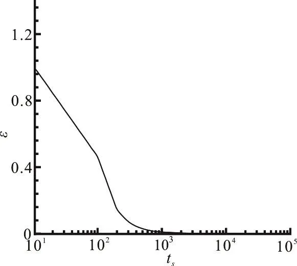
Fig. 13 Variations of maximal relative residual against time step when NO reaction is calculated in a straight vessel

4. Discussions

Based on the maximal relative residual of the NO concentration for all nodes against the time step, we select the current time step for the check of convergence of the NO auto-oxidation reaction in the whole domain. The calculated NO concentration is considered to be convergent if the maximal relative residual of all nodes is less than10-9. Figure 13 shows the maximal relative residual, denoted by ε, against the time steps (ts) when the NO reaction is calculated in a straight vessel under the condition of Lp=1.0×10-10m/Pa· s . With the time step marching from 10 to 105, the maximal relative residual decreases from 1 to 10-9. It is seen that the maximal relative residual rapidly decreases at the initial time period from 10 to 103indicating that the computation of the NO concentration can reach a stability state rapidly. The same convergence criterion is employed for the NO concentration computation in other structures as well.

On the other hand, the selection of the relationship between RNOand WSS is of importance in computing the NO distribution in the whole model.An increasing number of studies were carried out to explore the pathways that leads to the production of the NO in response to the WSS[16]. Currently, there are three relationships, proposed to describe the WSS-dependent NO production rate RNO, which are the linear model (RNO=Rbasal+Aτ), the sigmoidal model (RNO=Rmax/(1+Ae-Bτ)), and the hyperbolic model (RNO=Rbasal+Rmaxτ/(τ+A)). Kanai et al.[26]proposed a linear relationship between the NO production and the WSS in the range of 0.2-1.0 Pa.Using electrodes in the flow environment, Allison et al.[21]measured the real-time NO concentration levels produced by the endothelial cells exposed to controlled changes of the shear stress directly and they found that the hyperbolic model provided the closest match to the experimental date. We thus employ the hyperbolic model to calculate the WSS-dependent RNOin this study owing to the fact that the WSS value in this study is larger than1.0 Pa.

From Fig. 6(b), it is seen that the maximum value of the NO concentration in the vascular wall is about 3 nM when Lpand krbcare 10-10m/Pa·s and 23 s-1. In this situation, RNOis 200 nM·s-1as calculated by the hyperbolic model with the WSS taken the value of 2.5 Pa(Fig. 6(a)). According to Eq. (27), the product of the NO production rate RNOand the endothelial thickness is employed to reflect the secreted quantity of the NO, whose concentration is 0.4 nmol/m2s. Hood et al. provided a measured value of the NO production rate for the human umbilical vein endothelial cells,which is 417 nM·s-1obtained by an in-vitro experiment. The magnitude of RNOcalculated by our model is about half of the value measured by Hood et al.. Liu et al.[15]simulated the NO distribution at the lumen-wall interface of a straight artery using the hyperbolic model and the variation tendency calculated by Liu is in a good agreement with ours(Fig. 6). Additionally, the maximum NO concentrations in the lumen-wall interface calculated by Liu are about 3 nM and 6 nM when the values of krbcare 23 s-1and 2.3 s-1respectively. The maximum NO concentrations in the vascular wall calculated by our model are 3 nM and 8 nM when krbcare 23 s-1and 2.3 s-1, respectively, in the same order as Liuʼs results(Fig. 6). Meanwhile, the magnitude of the NO concentration obtained by our model is supported by the work of Palmer et al., where they found that the NO concentration is expected to be in nano to micro molar concentration levels.

Currently, a wide varieties of the values of the NO production rate RNOwere employed in different models and experiments. Lu et al.[27]measured the porcine carotid artery with a 2.5 ml/s flow and estimated that the NO production rate in their experiments was 3-12 μΜ/s. In the simulation of Tsoukias et al.[14], they employed the value of the production rate RNOof 13.25 μΜ/s , as in agreement with Luʼs experimental data under the condition when the thickness of the endothelium is 2 μm. The simulated maximum NO concentration in a capillary wall by Tsoukias et al. is about 25 nM in case of a large reaction rate with the RBCs (=3× 105s-1).Similarly, Vaughn[13]used a much larger RNO(26.5 μΜ/s)to simulate the NO transport in and around the arteriole and obtained the value of the NO concentration in the vascular wall as 270 nM in case of krbc=15s-1. In summary, compared to the available data, the computed NO concentration by our model is in the reasonable range of physiology.

The WSS distribution along the vascular wall reflects the change of the velocity gradient. For example, Lai et al.[28]pointed out that the maximal WSS occurs at the jet impinging point on the wall where the local velocity gradient is higher than those in other places. In our work, near the entrance of the capillary, the WSS increases with the rising of the hydraulic permeability due to the velocity gradient as shown in Fig. 6(a). However, near the exit of the capillary, the WSS decreases with the rising of the hydraulic permeability under the condition of Lp≤10-7m/Pa· s . It is worth noting that the WSS sharply increases at the exit of the vascular lumen when there is a reversal flow. Equation (14) shows that the hyperbolic variation of RNOensures that the endothelial NO production could not increase infinitely. As the WSS increases, the gradient of RNOdecreases in an exponential manner. Thus, the variation of the RNOlevels off when the WSS increases to a certain value. However, the influence of convection in the vessel lumen can counteract the NO production.Therefore, a balance is reached between the enhanced NO production and the increased convective influence when the WSS increases, leading to a non-monotonic relationship between the endothelial NO variation and the WSS. The conclusion of our simulation agrees very well with that summarized by Plata[17].

The diffusion of the NO along the radial direction plays an important role in influencing the NO distribution in the whole domain. The NO concentration profile along the radial direction is determined partly by the NO mass diffusion. In addition, the velocity field also has a significant impact on the NO concentration profile in the vascular lumen and the tissue. In the case of the same osmotic pressure, a faster transmural velocity induced by a larger hydraulic permeability permits more NO flow into the tissue. Thus, with a great increase of the vascular permeability, the NO distribution in the radial direction sees a significant difference.

It is generally believed that the NO enjoys many properties to induce the hemocytes to response and regulate the blood flow in the microcirculation. It can be seen from the results that with the NO transport in the straight and bifurcated vessels, the NO concentration in the domain experiences a clear decline due to the increase of the hydraulic permeability,especially in the region near the exit, which implies that the microvessel lesion is apt to occur in the domain near the exit of the capillary as the hydraulic permeability is larger there. It is interesting to note from Fig. 12 that that there is a fast increase of the NO concentration in the vessel lumen after the bifurcation,which was not observed in the work of Chen[11]. In their work, only the influence of the RBCs on the NO concentration was considered, but not the convection.

The spatial NO distribution may contribute to the determination of the local microangiopathy. For example, the low concentration area of the NO in a capillary may have an enhanced vascular permeability to the protein and the water because a significant feature of the NO is to regulate the permeability of the microvessel through leukocyte-dependent and independent mechanisms.

5. Conclusions

In the present study, we employ the FEM to simulate the NO transport with different hydraulic permeabilities in the system of the permeable capillary and the tissue. The simulation with the model demonstrates that the increasing permeability coefficient of the vascular endothelium can lead to a significant decrease of the NO concentration. On the other hand,the existence of branching can lead to a considerable increase of the NO concentration in the main capillary after bifurcation, which suggests that the NO concentration is not only dependent on the WSS but also on the convection inside the vessel.

Many experiments show that the hydraulic permeability of the endothelium increases for patients with the DM[1]. Our results may provide some new insight for exploring the change of the blood flow in the microcirculation in the case of the DM. Besides the variation of the vascular permeability, some hemorheological parameters may change in patients with the DM, including the enhanced erythrocyte aggregation and the reduced erythrocyte deformability.These parameters can influence the consumption of the NO in the blood. In the next step, we will combine our model with a model of the red blood cells to simulate the NO transport in the case of the hemorheological disorders in patients with the DM. In this process, the influence of the red blood cells on the micro-capillary flow is of importance[29]. Owing to the advances of the microfluidic techniques, the endothelial function induced by the WSS and the interaction between the endothelial and smooth muscle cells can be simulated in vitro[30-31]. With the help of these techniques, the behavior of the NO transport in patients with the diabetic mellitus can be further revealed, which will provide useful knowledge for early diagnostics of the DM vascular complications.

Acknowledgements

This work was supported by the Dalian Science and Technology R & D Program (Grant No.2015F11GH092), the Scientific Research Foundation of Liaoning Education Department (Grant No.L2015113).