Possible Sources of Forecast Errors Generated by the Global/Regional Assimilation and Prediction System for Landfalling Tropical Cyclones.Part II:Model Uncertainty
2018-08-14FeifanZHOUWansuoDUANHeZHANGandMunehikoYAMAGUCHI
Feifan ZHOU,Wansuo DUAN,He ZHANG,and Munehiko YAMAGUCHI
1Laboratory of Cloud-Precipitation Physics and Severe Storms,Institute of Atmospheric Physics,Chinese Academy of Sciences,Beijing 100029,China
2State Key Laboratory of Numerical Modeling for Atmospheric Sciences and Geophysical Fluid Dynamics,Institute of Atmospheric Physics,Chinese Academy of Sciences,Beijing 100029,China
3International Center for Climate and Environment Sciences(ICCES),Institute of Atmospheric Physics,Chinese Academy of Sciences,Beijing 100029,China
4Meteorological Research Institute of the Japan Meteorological Agency,Tsukuba 305-0052,Japan
5University of Chinese Academy of Sciences,Beijing 100049,China
ABSTRACT This paper investigates the possible sources of errors associated with tropical cyclone(TC)tracks forecasted using the Global/Regional Assimilation and Prediction System(GRAPES).In Part I,it is shown that the model error of GRAPES may be the main cause of poor forecasts of landfalling TCs.Thus,a further examination of the model error is the focus of Part II.Considering model error as a type of forcing,the model error can be represented by the combination of good forecasts and bad forecasts.Results show that there are systematic model errors.The model error of the geopotential height component has periodic features,with a period of 24 h and a global pattern of wavenumber 2 from west to east located between 60°S and 60°N.This periodic model error presents similar features as the atmospheric semidiurnal tide,which reflect signals from tropical diabatic heating,indicating that the parameter errors related to the tropical diabatic heating may be the source of the periodic model error.The above model errors are subtracted from the forecast equation and a series of new forecasts are made.The average forecasting capability using the rectified model is improved compared to simply improving the initial conditions of the original GRAPES model.This confirms the strong impact of the periodic model error on land falling TC track forecasts.Besides,if the model error used to rectify the model is obtained from an examination of additional TCs,the forecasting capabilities of the corresponding rectified model will be improved.
Key words:GRAPES,error diagnosis,model uncertainty,predictability,tropical cyclone
1.Introduction
Although the forecasting of tropical cyclone(TC)tracks has been improved notably in recent decades,large track forecast errors still exist for some TCs.The improvement of TC track forecasts is a longstanding concern.Currently,as the theory of TC motion is mature and widely accepted(Chan,2010),error diagnosis has become an important way to further improve TC track forecasts(Galarneau and Davis,2013).
Many studies have examined factors that may cause large forecast errors in TC tracks.These studies have found that TC track errors can arise from an erroneous forecast of the environmental winds(Brennan and Majumdar,2011),or of storm structure or intensity(McTaggart-Cowan et al.,2006),and these forecast errors can be traced back to errors in the initial conditions of the model(Komaromi et al.,2011),or bad representations in the model of the physical processes known to contribute to TC motion(Kehoe et al.,2007).Carr and Elsberry(2000a,b)also found that TC position errors in the Navy Operational Global Atmospheric Prediction System model and the Geophysical Fluid Dynamics Laboratory hurricane model are commonly driven by errors in TC or mid-latitude cyclone size and separation distance.Galarneau and Davis(2013)studied the TC position forecast errors that result from the definition of the steering flow.They suggested that an optimal steering layer depth and an optimal TC removal radius for each TC should be first found when using the steering flow to forecast TC tracks.
The uncertainties associated with models are another source of TC track forecast errors.For instance,it has been shown that the physical parameterization schemes chosen in a model’s configuration has a significant impact on its TC forecasts(Miglietta et al.,2015).Among them,the cumulus parameterization scheme has the greatest impact,while the boundary layer schemes and land-surface models appear to play only a marginal role.Kepert(2012)compared the simulation results from several boundary layer parameterization schemes with observations,and recommended the use of the Louis boundary layer scheme and a higher-order closure scheme for TC simulation.Green and Zhang(2014)examined the sensitivity of TC simulations to parametric uncertainties in air–sea fluxes by varying four key parameters,and found that both the intensity and the structure of TCs are highly dependent upon the two multiplicative parameters,suggesting that these parameters could be estimated by assimilating near-surface observations.
In an actual forecast,errors usually result from uncertainties in the model and in the initial conditions.However,if we can identify which type of uncertainty results in larger forecast errors,we can focus on that,and a substantial improvement can then be expected.
In Part I,the ability of the Global/Regional Assimilation and Prediction System(GRAPES)Global Forecast System(GRAPES_GFS)to forecast land falling TCs is examined,revealing that the model error associated with GRAPES_GFS(hereafter,GRAPES)forecasts may be the main cause of poor forecasts of land falling TCs.As a result,we further examine the source of model errors in Part II.
There are several ways to explore model errors.A popular approach is to test the sensitivity of the forecasts to different physical parameterization schemes,as previously introduced in the works of Miglietta et al.(2015)and Kepert(2012).Another common method is to selectively perturb the parameters in some of the schemes(Green and Zhang,2014).Recently,Sun and Mu(2017)proposed a method that can find the largest impacts of the parameters based on the conditional nonlinear optimal perturbation related to the parameter(CNOP-P),and they found that the nonlinear interactions among parameters play a key role in identifying the sensitive parameters.As a result,the most important parameter is different from that obtained by examining the impacts of parameters separately.However,the calculation of CNOP-P is computationallyvery expensive when applied to a complex model with a large number of parameters.In addition to the physical parameterization schemes and the parameters,model errors also derive from the discretization of the finite difference scheme and the accuracy of the computer. The effects of these model errors are mixed,making it difficult to distinguish the role of each type of model error in yielding prediction uncertainties.Duan and Zhou(2013)introduced a nonlinear forcing singular vector(NFSV)approach to approximately describe the combined effect of different types of model errors.An NFSV is the tendency error that generates the notable prediction error within a nonlinear model during a predetermined forecast period,and it can be roughly identified as responsible for processes that are omitted or mistreated by the model system.Duan and Zhao(2015)and Duan et al.(2016)used the NFSV approach to explore the role of model error in causing the so-called “spring predictability barrier”related to El Nino events.In this study,we adopt a similar approach to investigate the combined effects of different types of model errors,and then identify a simple and efficient way to reduce the model errors.
The structure of Part II is as follows:Section 2 outlines the method and experimental design.Section 3 presents the features of model errors and confirms their impacts on the forecasts using the results from hind casting experiments.A summary and discussion finalize the paper in section 4.
2.Methods
2.1.Error diagnosis
As mentioned in the introduction,we use tendency errors to approximate the combined effect of different types of model errors.In the following,we present how the model errors are diagnosed in the form of tendency.
The evolution equations for the state vector U can be written as


where Mtpropagates the initial value to the prediction time t.
Errors relating to both the initial conditions and the model itself exist in a realistic forecast system.To evaluate the impacts of initial condition errors on the forecasts,a common approach is to superimpose an initial perturbation on the initial conditions of the numerical model.Meanwhile,to investigate the effect of model errors on the prediction results,it has been suggested to superimpose a tendency perturbation on the right-hand side of the evolution equation,Eq.(1)(Roads,1987;Moore and Kleeman,1999;Barkmeijer et al.,2003;Duan and Zhou,2013).
A forecast model that describes both initial perturbations and tendency perturbations can be written as
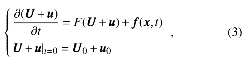

Here,we consider the second type of predictability problem—that is,the initial condition errors are set to zerowritten as

Considering the model errors but ignoring the initial condition errors,the discrete form of Eq.(3)can be presented as
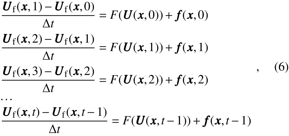
and
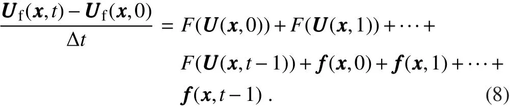
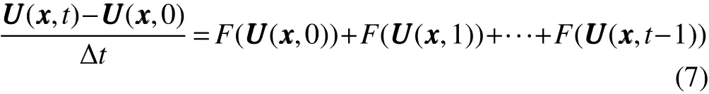
Subtracting Eq.(7)from Eq.(8),we obtain
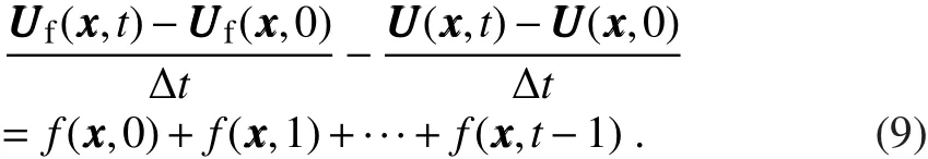
Equation(9)can be generalized to
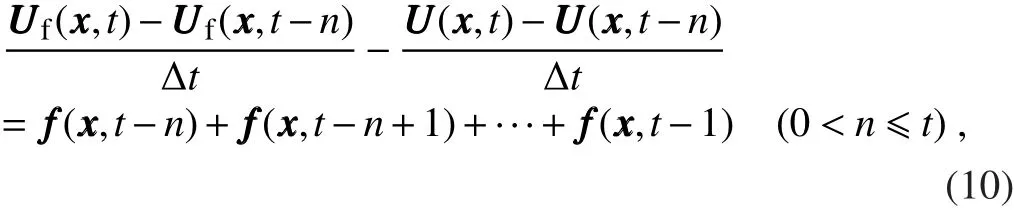
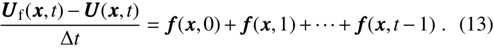
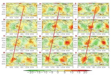
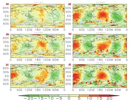
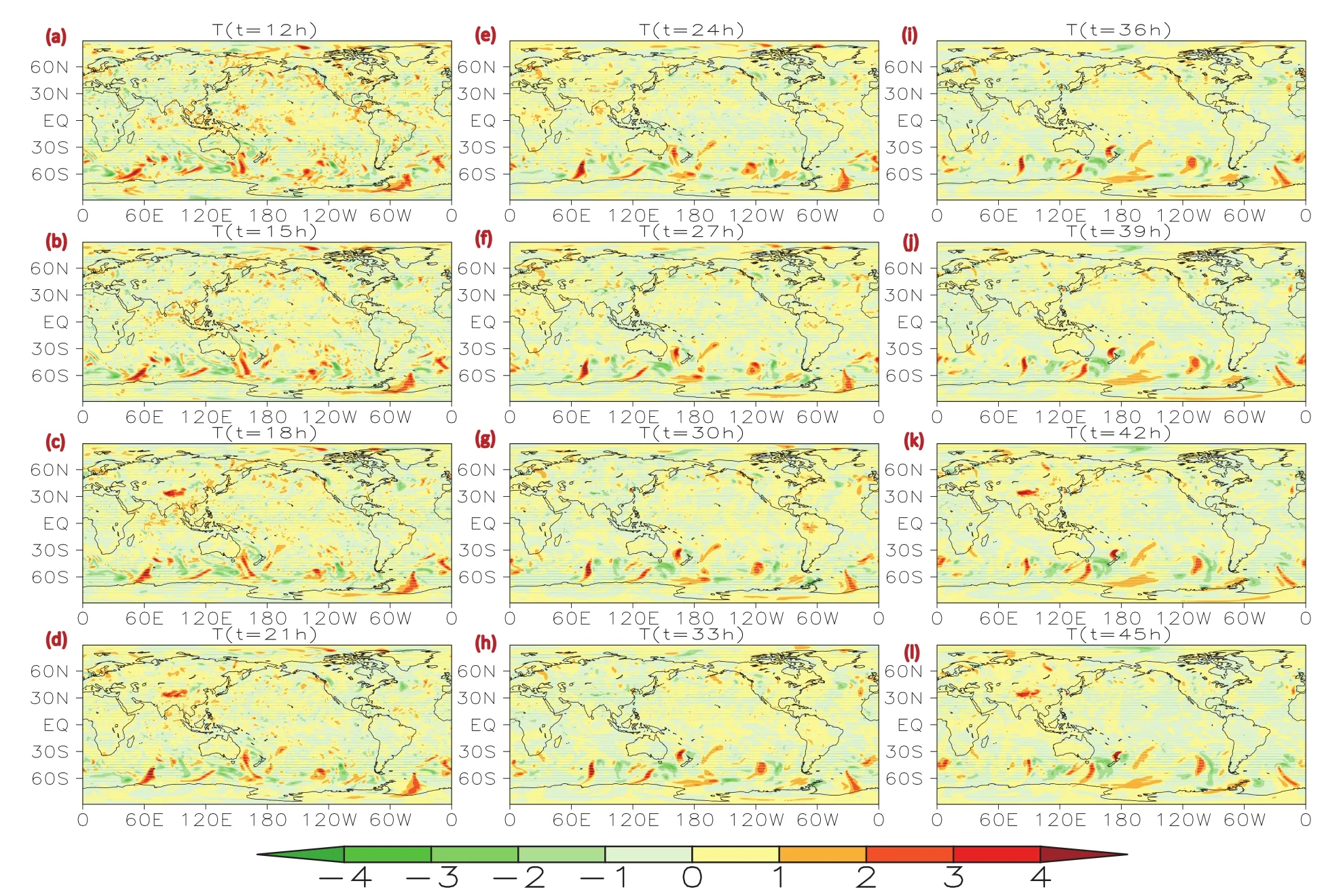
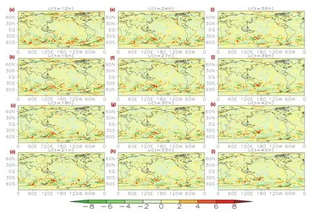
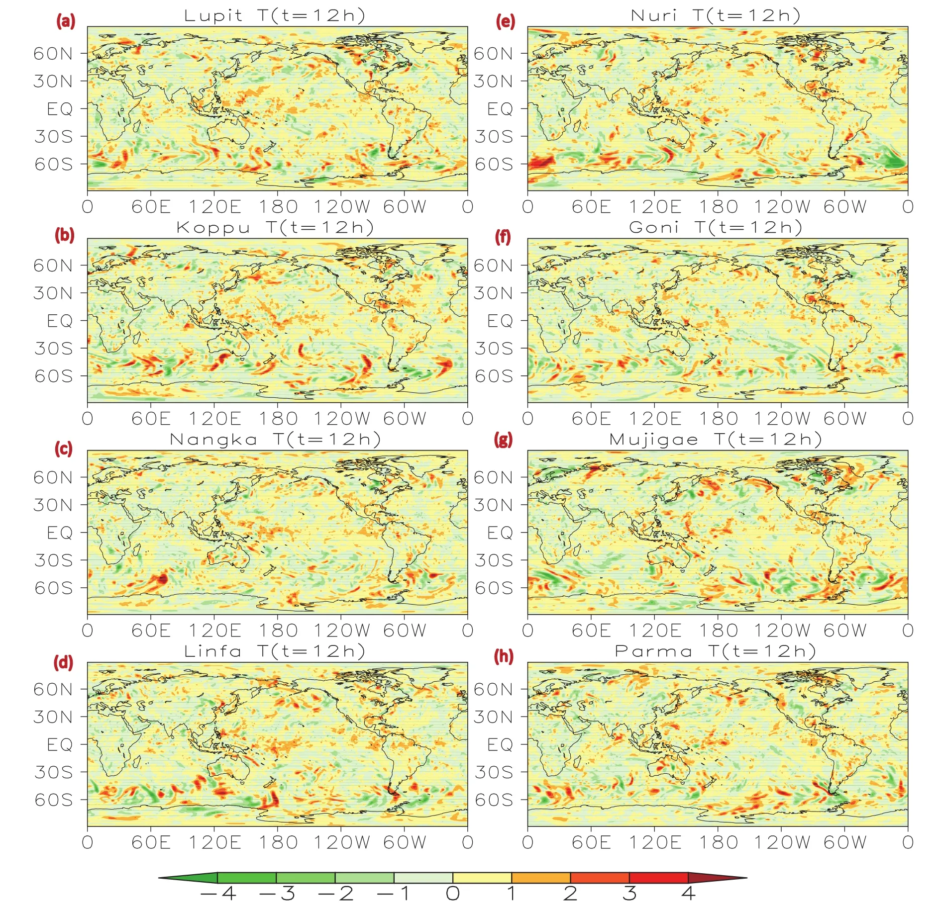
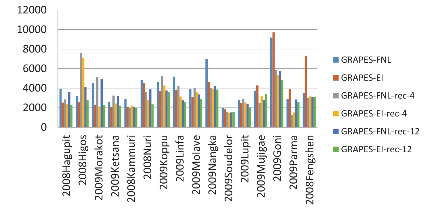
where n is the real number that satis fies 0 According to Eq.(11),if an accurate forecast or a high-systematic model errors at each time step t.If the output of the forecast is not known at each time step,e.g.,outputs at every 180 steps,according to Eq.(10)we can obtain the cumulative effect of model errors every 180 steps.By de finingEq.(10)can be written as Also of note is that the initial conditions of the perfect model[Eq.(1)]and the initial conditions of the imperfect model[Eq.(3)]are assumed to be the same.That is, Equation(13)indicates that the differences between the state vector at time t obtained from the imperfect model and the state vector at time t obtained from the perfect model reflect the cumulative effects of model errors from the initial time to time t. In this study,the GRAPES model is used to forecast 16 TCs that occurred in 2008 and 2009 in the West Pacific.In Part I(Zhou et al.,2016),it is found that the forecasts of these landfalling TCs are poor,and the model error may be the main cause.This indicates that the GRAPES model may have defects.In Part II,In Part II, we consider GRAPES as an imperfect model,and its forecasts are described as the state vectorIn Part I,it is demonstrated that the forecasts of the ECMWF model are generally good.Thus,in this study,we take the ECMWF model as the perfect model,and the initial conditions of the ECMWF model are assumed to have no errors.We mark the forecasts of the ECMWF model with the stateat each time step,we can obtain the systematic model error The following describes the design of the GRAPES model and introduces the dataset that supplies the forecasts of the ECMWF model.The horizontal resolution of GRAPES is 1°×1°,and there are 36 levels in the vertical direction.The physical parameterizations of GRAPES include the WSM6 scheme formicrophysics(Hong andLim,2006),the RRTMG(Iacono et al.,2008)scheme for longwave and shortwave radiation,the COLM(Dai et al.,2003)scheme for the land surface processes,the MRF(Hong and Pan,1996)scheme for the planetary boundary layer,and the simple Arakawa–Schubert(Han and Pan,2011)scheme for the cumulus cloud.The default initial conditions of GRAPES are supplied by the National Centers for Environment Predictions(NCEP)FNL(Final)Operational Global Analysis(1°×1°)interpolated into the GRAPES model.However,in our experiment,the default initial conditions are replaced with the initial conditions of the ECMWF model.The ECMWF model’s forecasts of the TCs in 2008 and 2009,as well as the initial conditions of the forecasts,can be downloaded from the Year of Tropical Convection(YOTC)dataset(http://www.wmo.int/pages/prog/arep/wwrp/new/yotc.html).Because GRAPES is a global model,its resolution cannot be adjusted.Consequently,we download the YOTC dataset with a horizontal resolution of 1°,equivalent to that of GRAPES.The output of the forecasts of the ECMWF model is saved every three hours.Therefore,we save the output of GRAPES every three hours too.The time step of GRAPES is 600 seconds,meaningthe output of GRAPES is saved every 18 steps.Therefore,we cannot calculate the model errors of GRAPES at each time step using Eq.(11),but we can calculate the model errors of GRAPES every 18 steps(every three hours)according to Eq.(12).To summarize,what we obtain are the cumulative model errors every 18 steps(every three hours).So,if t indicates the integration time step,then n=18 in Eq.(12);if t indicates the integration time period,then n=3 in Eq.(12). In the following,the forecasts by GRAPES with initial conditions of the ECMWF model are denoted as GRAPES_EI,and the forecasts by ECMWF with the same initial conditions are denoted as ECMWF_EI.The track data from the Chinese “Typhoon Online”website are considered as the true(observed)values(www.typhoon.org.cn;Ying et al.,2014). In this study,a total of 16 TCs that made landfall in 2008 and 2009 are considered(Table 1).In each case,forecasts are obtained 72 h before making landfall.In Part I,it is shown that,due to the marked improvement in position forecasting capability when replacing the initial conditions of GRAPES with those of the ECMWF model,4 of the 16 cases are identifiable as TCs whose position forecast errors are attributable to the initial condition errors;and due to the negligible or complete absence of improvement in position forecasting capability when renewing the initial conditions of GRAPES,12 TCs are identifiable as TCs whose position forecast errors are attributable to the model errors.The improvement rates(IM)are given in Table 1,and a threshold value of IM=0.5 is used to differentiate between initial error cases and model error cases.Thus,in this part,for convenience,we refer to the first type of TCs as initial-error-determined TCs,and the other type as model-error determined TCs.Next,we begin by examining the model errors that exist in every TC;then,we explore their common aspects,before finally rectifying the model errors and demonstrating the improvements following this revision. From Table 1,four of the TCs(Goni,Mujigae,Fengshen,Parma)show no improvement when replacing initial conditions from the FNL analyses with ECMWF analyses;thus,it is thought that the model errors are notable when forecasting these four TCs.We therefore refer to these four TCs as notable model-error-determined TCs,and the model errors associated with them are diagnosed first. Table 1.Summary of the TCs studied in this paper.The initial time is the start of the 72-h forecast.The improvement rates(IM)are calculated(only for the improved cases)using the equation IM=[(−)−(−)]/[−],where E indicates the departure of the forecast from the observations(the 72-h accumulated track errors calculated every six hours)and the subscripts indicate the various forecast errors.The forecasts by GRAPES with its default initial conditions is denoted as ,while the forecasts by GRAPES with initial conditions of the ECMWF model is denoted as ,and the forecasts by ECMWF with the same initial conditions is denoted as ECMWFEI. Table 1.Summary of the TCs studied in this paper.The initial time is the start of the 72-h forecast.The improvement rates(IM)are calculated(only for the improved cases)using the equation IM=[(−)−(−)]/[−],where E indicates the departure of the forecast from the observations(the 72-h accumulated track errors calculated every six hours)and the subscripts indicate the various forecast errors.The forecasts by GRAPES with its default initial conditions is denoted as ,while the forecasts by GRAPES with initial conditions of the ECMWF model is denoted as ,and the forecasts by ECMWF with the same initial conditions is denoted as ECMWFEI. Category Name Initial times IM value Initial-error- Higos 1200 UTC 1 Oct 2008 0.55 determined Hagupit 1200 UTC 20 Sep 2008 0.51 Morakot 1200 UTC 4 Aug 2009 79.9 Ketsana 1200 UTC 25 Sep 2009 1.32 Model-error- Lupit 1200 UTC 21 Oct 2009 0.16 determined Kammuri 1200 UTC 4 Aug 2008 0.44 Nuri 1200 UTC 18 Aug 2008 0.08 Linfa 1200 UTC 18 Jun 2009 0.38 Nangka 1200 UTC 23 Jun 2009 0.43 Koppu 1200 UTC 12 Sep 2009 0.33 Soudelor 1200 UTC 10 Jul 2009 0.16 Molave 1200 UTC 16 Jul 2009 0.33 Fengshen 1200 UTC 21 Jun 2008 –Mujigae 1200 UTC 9 Sep 2009 –Goni 1200 UTC 1 Aug 2009 –Parma 1200 UTC 30 Sep 2009 – Figure 1 shows the global distribution of the model errors of geopotential height at 500 hPa at forecast times of 12 h to 45 h(with an interval of 3 h)diagnosed from the forecasts of TC Fengshen.The model errors have north–south zonal banded distributions.From 60°S to 60°N,the positive errors and negative errors appear alternately from west to east.The patterns at 12 h,24 h,and 36 h are similar,as the positive errors appear from about 30°W to 60°E,and from 150°E to 120°W.Meanwhile,the positive model errors at 15 h,27 h,and 39 h are located slightly west compared to those at 12 h,24 h,and 36 h,respectively.At these times,the positive errors are located at about 60°W to 30°E,and at 120°E to 150°W.The positive errors move further west at the forecast times of 18 h,30 h,and 42 h,and are located at about 60°E to 150°E and about 120°W to 30°W.The positive errors again move westward at the forecast times of 21 h,33 h,and 45 h,meaning they are now located at 30°E to 120°E and 150°W to 60°W.As time progresses to 48 h,the distributions of the patterns are identical to those at 12 h.Indeed,the positive errors located at about 150°E to 120°W at the forecast time of 12 h catch up with those primarily located at about 30°W to 60°E at the forecast time of 24 h,before then returning to the previous position when the forecast time is 36 h.This circular pattern continues with a period of 24 h.Figure 2 shows the distributions of the model errors of geopotential height at 500 hPa at forecast times from 12 h to 72 h with an interval of 12 h.The patterns are similar,meaning that every 12 h the model errors present the same pattern.However,notably,the model errors vary periodically with a periodicity of 24 h,which is a favorable regularity that it is easy for us to overcome. This periodic regularity of the model errors can be diagnosed not only from these four notable model-errordetermined TCs,but also from all other model-errordetermined TCs( figures not shown).Even more encouraging is that the model error patterns diagnosed from all cases present high levels of similarity.For example,the positive errors are all located at about 30°W to 60°E,and from 150°E to 120°E,at the forecast time of 12 h(Fig.3).Likewise,at the forecast time of 15 h they are all located at about 60°W to 30°E and at 120°E to 150°W(Fig.4),and so on. Clearly,this periodic distribution of the model errors is case-independent,and thus inherent to the model.It is a real model error that is easy to rectify due to its periodicity. In addition,there are randomly exhibited model errors in the wave-like flows at 60°S in the Southern Hemisphere(Figs.1–4).Unlike the previously mentioned periodic errors,these errors are on a small scale,propagate eastward with wave-like flow,move much slower,and have a short duration(Figs.1 and 2).They usually appear at the trough of the basic flow,then move downstream and,after a period of growth,decay gradually and die before reaching another trough.Since these model errors are far away from the typhoons and their durations are short,they may have only a small impact on the typhoon forecasts.From another perspective,because these model errors present different distributions from case to case(Fig.3),they may not be intrinsic model errors.Besides,their small-scale patterns and irregular distributions make them more like random errors,which makes them hard to rectify. Fig.1.Global distribution of geopotential height(contours;units:m;contour interval:200 m)and the model errors of geopotential height[shaded;units:m(3 h)−1]at 500 hPa,at forecast times of(a)12 h to(l)45 h(every 3 h per panel)for the Fengshen case.The red line denotes the errors moving west. Fig.2.As in Fig.1 but at forecast times from(a)12 h to(f)72 h(every 12 h per panel)for the Fengshen case. The largest model errors for temperature and wind seem to be concentrated from 30°S to 60°S(Figs.5–7).Their behaviors are somewhat like those of geopotential height in this area.That is,both are small-scale,propagate eastward with the wave-like basic flow,move slowly,and have short durations.Similarly,these kinds of model errors present different distributions from case to case(Fig.7),meaning it is difficult to extract the common characteristics to be rectified.We hypothesize that because these model errors exist far from the typhoons,and their durations are short,they may have only a small impact on typhoon forecasts. According to the analysis in section 3.2,there are two notable phenomena of model error.One is the periodic model error that exists in the forecasts of geopotential height,with a period of 24 h.This model error exhibits a wave-like pattern(wavenumber 2)around the globe and is mainly concentrated between 30°S and 30°N.This type of error can be diagnosed from all TC forecasts,so it is deemed to be an intrinsic model error.The other type of error is the small-scaled model error located from 30°S to 60°S that exists in the forecasts of all variables.However,because this kind of model error presents different distributions from case to case,they are more like random errors and hard to rectify.They are located in the westerly jet over the Southern Hemisphere,and possibly triggered by the departure of the wind simulations in that region.It has been reported that the wind there is difficult to simulate well(Swart and Fyfe,2012).In this section,we focus on the systematic errors of the first kind(namely,the periodic model error),and discuss its possible source. With regard to the source of periodic model errors,we find that they present similar features to the atmospheric semidiurnal(S2)tide.Atmospheric tide is the dynamical response to periodic diabatic heating(Chapman and Lindzen,1970),and the S2 tide is a predominant component of atmospheric tides that prevails in the tropics(Sakazaki and Hamilton,2017).The S2 tide can interact with the mean flow through convective precipitation(Woolnough et al.,2004),and thus in fluences the weather systems that occur in the tropics.Hotta et al.(2013)pointed out that the tidal signals can effectively reflect signals from tropical diabatic heating,which is considered to be the most significant source of model uncertainty,and thus the discrepancy in atmo-spheric tides between the model and observation might give us some information about model errors.They conducted an intercomparison of S2 tides in TIGGE(The International Grand Global Ensemble)models,and found that not all models are successful in representing them.The S2 tides in the ECMWF model are consistent with observations,while those in the China Meteorological Administration’s global model are much weaker than their counterparts in the ECMWF model,and show a phase shift.Combined with our work,this result suggests GRAPES is ineffective at representing the S2 tides.Since the S2 tides can reflect signals from tropical diabatic heating,this means that GRAPES does not perform well in describing the tropical diabatic heating.Thus,the parameters or physical processes that are related to the tropical diabatic heating deserve closer attention.Some studies have also pointed out that the absorption of shortwave radiation by ozone triggers the greatest meridionally symmetric mode for the migrating S2 tide,and at low latitudes this forcing explains about 70%of the amplitude of S2 tides;whereas,the absorption of longwave radiation by water vapor in the troposphere explains 20%of amplitude,and the latent heating associated with tropical convection explains about 10%(Butler and Small,1963;Chapman and Lindzen,1970).Lindzen(1978)pointed out that,although the contribution from latent heat is small,it significantly affects the phase.Sakazaki and Hamilton(2017)used a comprehensive numerical model to verify the theory of the importance of the latent heat on the phase of S2 tides.From the above studies,it is speculated that the parameters(or parameterization schemes)related to the tropical diabatic heating including the shortwave absorption,longwave absorption and latent heat in the GRAPES model may have defects,which may be the source of the periodic model errors presented above. Fig.3.Global distribution of geopotential height(contours;units:m;contour interval:200 m)and the model errors of geopotential height[shaded;units:m(3 h)−1]at 500 hPa,at the forecast time of 12 h for eight TC cases:(a)TC Lupit;(b)TC Koppu;(c)TC Nangka;(d)TC Linfa;(e)TC Nuri;(f)TC Goni;(g)TC Mujigae;(h)TC Parma. Fig.4.As in Fig.3 but at the forecast time of 15 h for eight TC cases:(a)TC Lupit;(b)TC Koppu;(c)TC Nangka;(d)TC Linfa;(e)TC Nuri;(f)TC Goni;(g)TC Mujigae;(h)TC Parma. The results presented in section 3.3 suggest that revising the parameters(or parameterization schemes)related to the tropical diabatic heating could be one way to improve the TC track forecasts produced by the GRAPES model.However,before this revision,a series of sensitivity experiments regarding the parameters or parameterization schemes need to be conducted,and this requires a lot of work.Instead,we adopt a simpler and more efficient way to improve the TC track forecasts.Since the periodic model error is obtained in the form of tendency error,we can thus subtract it from the model equations directly.Then,an improved model can be obtained.In the following,we describe the detail of the experiments and their corresponding results. In Part I,it is shown that there are four TCs whose forecasts do not improve despite improvement in their initial conditions.Therefore,the model errors in these four TCs are notable.Accordingly,we first use the information on the model errors diagnosed from these four TCs to rectify the model.Since the periodic model errors have the same period and similar patterns,we average them and use the averaged model errors to rectify the model and then produce forecasts.Specifically,the averaged model errors are taken as the negative tendency perturbations in Eq.(3)or Eq.(6)in discrete form in the forecasts of geopotential height.Since the model errors are obtained every three hours,the negative tendency perturbations are added every three hours too in the model integration.All forecasts of the TC tracks are recalculated,and the new forecasts are named GRAPESFNLrec4.The results show that nine TCs are improved compared to the original forecasts(using the original GRAPES model and the FNL initial conditions—hereafter,GRAPES_FNL),while eight TCs are further improved compared to the forecasts that use the ECMWF initial conditions and the original GRAPES model(hereafter,GRAPES_EI)(Fig.8).If we only rectify the model but do not improve the initial conditions,the forecasts of the initial-determined TCs are not improved.However,the four TCs whose information is used show larger improvements than the others.The average forecast errors show that,regardless of whether we improve the initial conditions or the models,the largest benefits are obtained during the later forecast periods(Fig.9);and generally,reducing model errors results in more benefits compared with reducing initial errors(Fig.9). Fig.5.Global distribution of the temperature component of model errors[shaded;units:K(3 h)−1]at 500 hPa,at forecast times from(a)12 h to(l)45 h(every 3 h per panel)for the Fengshen case. Fig.6.Global distribution of the zonal wind component of model errors[shaded;units:m s−1(3 h)−1]at 500 hPa,at forecast times from(a)12 h to(l)45 h(every 3 h per panel)for the Fengshen case. Fig.7.Global distribution of the temperature component of model errors[shaded;units:K(3 h)−1]at 500 hPa,at the forecast time of 12 h for eight TC cases:(a)TC Lupit;(b)TC Koppu;(c)TC Nangka;(d)TC Linfa;(e)TC Nuri;(f)TC Goni;(g)TC Mujigae;(h)TC Parma. Because notable benefits are apparent when using the model error information obtained from just four TCs,it would be interesting to use information from additional TCs to rectify the model.Therefore,we next use the model error information diagnosed from 12 TCs that belong to the modelerror determined category of TCs.As before,we average them,and use this information to rectify the model,before producing a series of new forecasts calledThe results are highly encouraging.All the forecasts of the model-error determined TCs are obviously improved(Fig.8),with 10 that are further improved compared to theforecasts and the other two having comparable forecast capabilities with theforecasts.However,the four initial-determined TCs remain unimproved,which further confirms the importance of the initial conditions for those four TCs.The average forecast errors of all 16 TCs are reduced notably during the later forecast time periods.The improvement in the forecasting capabilities obtained from the reduction in model errors is nearly twice as much as that obtained from the reduction in initial errors during the later 36 h of the forecast period(Fig.9).This result indicates that if a model can be rectified based on a larger quantity of information diagnosed from numerous cases,it is possible to obtain a more reliable model that produces better forecasts than before its adjustment. Fig.8.Accumulated track errors(units:km;accumulated every 6 h with a total time period of 72 h)for each typhoon by the GRAPES model with its default initial conditions(GRAPESFNL)and with ECMWF initial conditions(GRAPES-EI),the revised GRAPES model with its default initial conditions(,),and the revised GRAPES model with ECMWF initial conditions(,).Theandparts of the names represent the model having been revised by subtracting the averaged model errors diagnosed from 4 TCs and 12 TCs,respectively. Fig.9.As in Fig.8 but for averaged forecast errors(units:km)of the 16 cases at 6-h intervals. Next,we further reduce the initial errors in the rectified model.As shown in Part I,the initial conditions generated from the ECMWF dataset(hereafter,EI)are generally better than those generated from the FNL data set(hereafter,FNL).So,here,we use EI to generate the initial conditions,and then use the rectified model to produce new forecasts.We refer to the rectified model obtained from adding the negative tendency perturbations deduced from four TCs asmodel,while that deduced from 12 TCs is referred to asmodel.The new forecasts from themodel with EI initial conditions are namedwhile the forecasts from themodel with EI initial conditions are namedWe find that by using EI to generate the initial conditions,whether with themodel or themodel,the forecasting capabilities are further improved compared with(Fig.9).If we take the difference between GRAPES FNL andas the improvement inthening capability,as the forecast error is the smallest,followedmeans that using more information to rectify the model,i.e.,the model is better presented(with either ECMWF or FNL initial conditions),is more beneficial.The rectified model using the FNL initial conditions generally has slightly inferior forecast capabilities compared to that using the EI initial conditions. Looking specifically at each individual case,for mostity(Fig.8),and the rectified model with initial conditions generated using EI has better forecasting capability than that with initial conditions generated using FNL.This is consistent with the averaged results shown in Fig.9.Clearly,the rectified model improves the forecast in most cases.However,for the four initial-determined cases,if we only rec-tial conditions,the forecasts are not improved and,in fact,worsen.This further confirms that they belong to the category of initial-determined TCs. Finally,it is found that for the initial-determined TCs,the model-error determined TCs,and the notable model-error determined TCs,most TCs have a bias toward the right-hand side of the observed track.This phenomenon has also been reported by Yamaguchi et al.(2012),using a model developed by the Japan Meteorological Agency.We can see that when reducing the initial errors or the model errors,the track shifts to the left of the original forecast track but remains to the right of the observed track(Fig.10).This indicates that there is another type of systematic error(yet to be identified)that leads to this phenomenon of a right-sided bias. Exploring the source of forecast errors is an important way to improve forecasts.In this second part of a two-part study,we focus on the source of the forecast errors that can be attributed to the model errors.Similar to the NFSV,the model error is taken as a type of forcing,which can be deduced by combining a good forecast with a well-developed model and a bad forecast with the model to be evaluated. It is found that the model errors of the geopotential height component have a periodic structure,with a period of 24 h.This wave-like and periodic-structured model error can be diagnosed from all TC forecasts.As it is located between 60°S and 60°N,and globally from west to east with awavenumber-2 pattern,it may be an intrinsic model error and have a notable influence on TC track forecasts.The model errors of the wind and temperature components turn out to be small-scale and situated a long distance from the TCs.Additionally,their durations are short.Since they are different from case to case,they are more like random errors.Thus,taking everything into account,they may have little influence on TCs. Fig.10.Tracks of(a)TC Hagupit,(b)TC Nuri(b),and(c)TC Fengshen.The black line indicates the observational track;the green line with a dot indicates the track forecasted by the GRAPES model with its default initial conditions(GRAPES-FNL);the green line with a cross or a vertical line indicates the track forecasted by the revised GRAPES model with its default initial conditions().Theandparts of the names represent the model having been revised by subtracting the averaged model errors diagnosed from 4 TCs and 12 TCs,respectively.The red lines are similar to the green lines but with ECMWF initial conditions. The periodic model error presents similar features to the atmospheric semidiurnal(S2)tide.Since the model errors are obtained from the deduction of the difference between the outputs of GRAPES and the ECMWF model,and the ECMWF model can successfully represent S2 tides,we hypothesize that GRAPES cannot represent the S2 tides well.Since the S2 tides reflect signals from tropical diabatic heating including the absorption of shortwave radiation by ozone,the absorption of longwave radiation by water vapor,and the latent heating associated with tropical convection,it is therefore speculated that the parameters or parameterization schemes related to the tropical diabatic heating may have defects,which result in the periodic model errors.However,this requires further investigation. The model is rectified according to the periodic model errors.First,the model is rectified using only the model error information diagnosed from four TCs identified as notable model-error determined TCs,and the corresponding ex-model is rectified using the model error information diagnosedfrom 12 TCs identified as model-error determined TCs,It is found that,for both experiments,the average forecast-iments improve the forecasts of the four notable model-error determined TCs considerably,but improve the forecasts ofan improvement that is nearly 1.5 times greater than that from simply improving the initial conditions.This indicates that the more information used to rectify the model,the greater the benefit.Furthermore,the initial conditions are also improved in the rectified model,and this further reduces theforecasting capability,with an improvement that is nearly 2.5 times greater than that obtained by simply improving the ini-with an almost twofold improvement over simply improving the initial conditions.An analysis of each individual case broadly confirms the averaged results. Generally,by rectifying the periodic model errors of geopotential height,the track forecasts of land falling TCs can be improved considerably,demonstrating the strong impact of periodic model errors on land falling TC track forecasts.However,the improved tracks also remain biased to the right of the track,indicating that another kind of systematic model error,yet to be identified,may exist. In this paper,model errors are diagnosed after the forecasts have been made,which of course seems unrealistic in a practical sense.However,if we can identify a model error that can be diagnosed from a specific kind of weather event,it is speculated that this model error will affect the model’s forecasts of the same type of weather in the future.Thus,if we can rectify the model error,we should then be able to improve the model’s forecasts of this type of weather.The model tendency error represents the overall effect of each type of model error.Rectifying the model using a negative tendency is a simple and effective way to improve forecasts of the specific type of weather event;however,it may fail to improve the forecasts of other types of weather.Therefore,identifying the source of the model tendency error is also necessary.This paper indicates that the parameters or parameterization schemes related to tropical diabatic heating may be the source of the periodic model tendency errors;however,to confirm this suggestion,numerous sensitivity experiments by model developers are required. Finally,it is important to note that the resolution of the model used in this study is only 1°,which is too coarse to discuss the behavior of TCs in depth.The forecasts of TC tracks produced by the GRAPES model only have indicative significance.High resolutions are necessary for a better representationof TC movement.In the study,we propose a method to identify the source of the forecast errors generated by the GRAPES model,and TCs are used as cases to show the application.With such a low resolution,the errors found are synoptic to global in scale.The next step will be to analyze the forecasts of TC tracks produced by other models with relatively higher resolution. Acknowledgements.We thank Dr.Daisuke HOTTA at the Meteorological Research Institute of the Japan Meteorological Agency for his assistance with the analysis of the source of systematic model errors.We thank the two anonymous reviewers for their helpful comments on the original manuscript.This research was jointly supported by the National Key Research and Development Program of China(Grant.No.2017YFC1501601),the National Natural Science Foundation of China(Grant.No.41475100),the National Science and Technology Support Program(Grant.No.2012BAC22B03),and the Youth Innovation Promotion Association of the Chinese Academy of Sciences.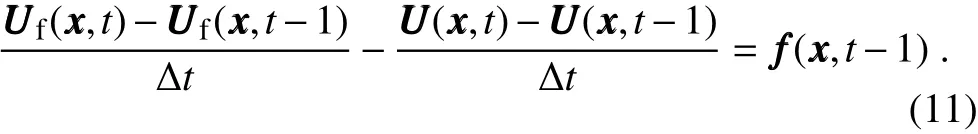

2.2.Experimental design
3.Results
3.1.Brief review of the TCs
3.2.Systematic errors in the model

3.3.Possible source of the systematic model errors


3.4.Adjustment of the forecasts by rectifying systematic model errors

4.Summary and discussion

杂志排行

Advances in Atmospheric Sciences的其它文章
- Circulation Features Associated with the Record-breaking Typhoon Silence in August 2014
- Investigating the Initial Errors that Cause Predictability Barriers for Indian Ocean Dipole Events Using CMIP5 Model Outputs
- Assimilation of Sea Surface Temperature in a Global Hybrid Coordinate Ocean Model
- High-Order Statistics of Temperature Fluctuations in an Unstable Atmospheric Surface Layer over Grassland
- Impact of Global Oceanic Warming on Winter Eurasian Climate
- A High-Resolution Modeling Study of the 19 June 2002 Convective Initiation Case during IHOP_2002:Localized Forcing by Horizontal Convective Rolls